AP MICRO U3 VOCABS
 Call Kai
 Learn
 Practice Test
 Spaced Repetition
 Match
 Flashcards
 Knowt Play
1/121

There's no tags or description
Looks like no tags are added yet.
122 Terms
Fixed resources
resources that DON'T change with the amount produced
Variable resources
resources that DO change as more/less is produced
Total Product (TP)
total output/quantity produced, avg product x labor
Marginal Product (MP)
the additional output generated by additional inputs (workers). Formula = 🔺TP/🔺inputs
Average Product (AP)
the output per unit of input.
Formula = TP/units of labor
Law of diminishing marginal returns
as variable resources (workers) are added to fixed resources (machinery, tools, etc), the additional output produced from each new worker will EVENTUALLY FALL.

Production function
shows the relationship between the quantity of inputs and the quantity of outputs.

long run
ALL inputs are available
short run
AT LEAST ONE input is fixed
fixed inputs
those inputs CANNOT be changed in the short run to change production (physical capital, factories, machines)
variable inputs
those inputs CAN be changed in the short run to change production (labor, certain materials/supplies)

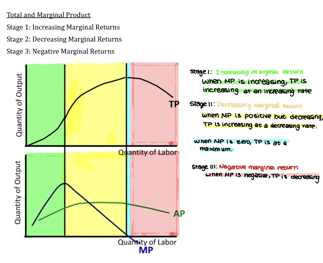
TP, AP, MP Graph
,,,,


Stage 1 of Total and Marginal Product
increasing marginal returns. when MP is increasing, TP is increasing at an increasing rate

Stage 2 of Total and Marginal Product
decreasing marginal return, when MP is positive but decreasing, TP is increasing at a decreasing rate


Stage 2.5(?) of total and marginal product
when mp is zero, TP is at a maximum


Stage 3 of Total and Marginal Product
negative marginal return, when MP is negative, TP is decreasing


MP crosses through the maximum of AP
when MP is above AP, AP is rising. When MP is below AP, AP is falling

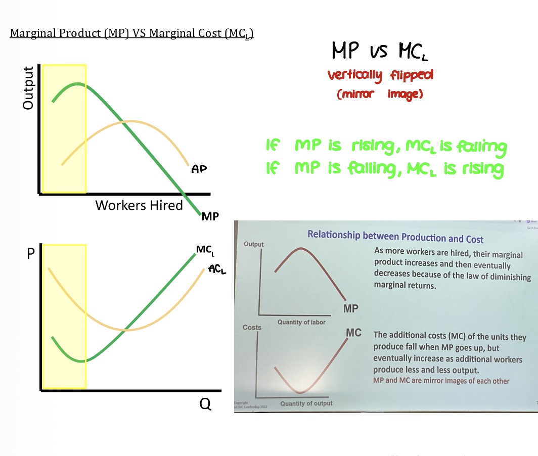
Marginal cost of labor (MC_L)
W/MP_L (wage / marginal product)

MP vs MC
If MP is rising, MC_L is falling; If MP is falling, MC_L is rising
Fixed costs
don't change with output (in short run); basically same cost regardless of changes (ex. rent, physical capital, land)

Variable costs
change with output(ex. labor, electricity, raw materials)

Total cost
FIxed cost + variable cost or (TFC + TVC)
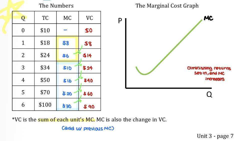
Marginal cost
The cost of producing the last unit.
Formula: 🔺TC/🔺Q (change in Q is usually 1)
VC & MC
VC is the sum of each unit’s MC. MC is also the change in VC

Average total cost (ATC)
TC/Q

Average Variable cost (AVC)
VC/Q
Average fixed cost (AFC)
FC/Q

Total variable cost (TVC)
TC-TFC or (AFC x Q)
Total fixed cost (TFC)
TC - TVC or (AVC x Q)

Finding costs
At Q1; MC = P1, AVC = P2, ATC = P3, AFC = P3-P2. AFC at any quantity is the gap between ATC and AVC

Finding total costs (with graph)
Average x Q. For Q1; VC = Q1 x P2, TC = Q1 x P3, FC = Q1 x (P3-P2)


Changing costs - shifting cost curves (increase in FIXED costs)
moves ATC only (does not move MC). EX = change in rent (INC), lump sum tax (INC), lump sum subsidy (DEC).


Changing costs - shifting cost curves (increase in VARIABLE costs)
moves ATC, AVC and MC. EX = changes in wages (INC), per-unit tax (INC), per-unit subsidy (DEC)

Key points
MC decreases at first (due to specialization and increasing MP) and then increases (due to diminishing returns and a decreasing mP)
ATC and AVC are U-shaped
MC crosses through the minimums of ATC and AVC
If MC is below ATC, then ATC is falling;if MC is below AVC, the AVC is falling.
If MC is above ATC, then ATC is rising; if MC is above AVC, then AVC is rising.
AFC is always decreasing, so AVC and ATC get closer together.
Cost curves shift if there are changes to input costs or productivity
Short run
at least 1 input is fixed; changes in rate of production
Long run
all inputs are available; changes in the capacity of production
examples of long run actions
chain opening a new franchise, a local restaurant can build an expanded dining room. a college can build a new dorm for more students, etc
Long run + more
long run decisions require heavy investment and expansion which are expensive, thus fixed costs will rise but workers will be more productive, so variable costs will fall.

Short run ATC graph
—--


Long-run ATC graph
—--

Economies of scale
long-run average total cost DECREASES as output INCREASES; can happen because of greater specialization of labor and/or better use of physical capital

diseconomies of scale
long-run average total cost INCREASES as output INCREASES; can happen because a firm gets so large that communication and supervision are more difficult and workers are less motivated (expanding -> problems)

constant returns to scale (efficient scale)
longrun average total cost is CONSTANT as output INCREASES

minimum efficient scale
the smallest plant capacity that allows a firm to minimize its ATC; helps to determine the concentration of firms in a market & the market structure

3-phases of long-run costs
Long-run average costs stay the same; 1. economies of scale, 2.constant returns to scale/efficient scale range, 3. diseconomies of scale

returns of scale
how much output increases in responses to the inputs used in the production process

increasing returns to scale
output is increasing at a faster rate than all inputs. doubles all inputs -> get more than double output (TCx2/Qx3 -> ATC decrease)


constant returns to scale
output is increasing at the SAME rate as all inputs. double all inputs -> get exactly double output (TCx2/Qx2 -> ATC is constant)


decreasing returns to scale
output is increasing at a slower rate than all inputs. double all inputs -> get less than double output (TCx2/Qx1.5 -> ATC increase)


various possible long-run ATC curves
___

Profit
TR-TC
Total Revenue (TR)
PxQ
Profit per unit (average profit)
Price - ATC or Econ Profit/Q
Explicit costs (accounting costs)
costs that are directly incurred by a firm (involve actually spending money)
Implicit costs (economic costs)
costs that don't involve paying money but rather are measured by the value of what is given up.
forms of implicit costs
Implicit cost of a business owner’s time/labor (salary from your next best alternate job), the implicit cost of physical or financial capital
Accounting profit
total revenue - explicit costs( accounting costs)
Economic profit
total revenue - explicit costs - implicit costs
(Econ profit is ALWAYS less than accounting profit)
Depreciation
lost in value of physical capital due to wear and tear over time => treated like an explicit cost
normal profit
when economic profit = $0, accounting profit = implicit costs ; means the business is no better off OR worse off than they would be in their next best alternative job
marginal revenue
the additional revenue earned from selling one more item; MR = changeTR/changeQ
marginal cost
the additional cost of producing one more item; MR=changeTC/changeQ
marginal profit
the additional profit earned from making and selling one more item; MR = changeP/changeQ or MR-MC
profit maximizing quantity rule
MR = MC; produce as long as MR>= MC but NEVER when MR<MC
Break-even point
P = ATC or TC = TR
Profit maximization on graph (constant MR) - at low quantity
MR>MC
Profit maximization on graph (constant MR) - at high quantity
MR<MC
Profit maximization on graph (constant MR) - profit maximization
MR=MC; produce up to last unit where MR>= MC
Profit maximization on graph
decreasing MR
Shut down
temporarily closing
exit the market
permanently closing
shut down rule
If TR < VC (or P <AVC), the firm should shut down
(shut down rule) If TR>TC or TR=TC
stay open; profit or break even
(shut down rule) if VC<TR<TC
stay open; operating at a loss
(shut down rule) If TR<VC<TC
shut down temporarily (cheaper to shut down)
profit
when MR = MC >= ATC
break-even
when MR = MC = ATC
operating at a loss, but stay open
when AVC < MR=MC < ATC
shut-down
MR = MC < AVC
When do you make a loss
When your ATC is ABOVE where your MR=MC
When do you make a gain/profit
When your ATC is BELOW where your MR = MC
per-unit measurements on graph
1) find where MR=MC -> P. max quantity , 2) compare P and ATC at Pmax to determine profits
in the long run, there are…
no fixed costs
if a firm is earning a loss in the long run…
will exit the market or industry
if firms are earning positive economic profit…
other firms will enter that market because there are profit making opportunities
barriers to entry examples
patent and copyrights, brand identity, government restrictions, start-up costs
long run
enter or exit has to do with profit and losses
market structure
how competitive it is
competitive scale (Least to most)
monopoly, oligopoly, monopolistic competition, perfect competition
how to determine market structure
1) how many firms are in the market, 2) do they produce a differentiated or a standardized (identical) product?
characteristics of perfect competition
many firms, identical products, low barriers to entry, no influence on price (all is zero long-run profit price takers) (ex. agriculture commodities, international currency markets)
MR=D=AR=P
average revenue
Average Revenue (AR)
TR/Q
side-by-side graph
market price extends to firm graph to form MR = D= AR=P
short-run profit graph
sds
short run loss (operating at a loss) graph
operate as long as P>AVC
draw long run break even (zero economic profit) graph
sds
profits
P>ATC
losses with still operating
AVC < P < ATC
shutting down
P < AVC