Checkpoint 3 (Alts, Portfolio Management)

Commodity Basis

Spot - Future

Commodity Calendar Spread

Futures Price of nearer maturity - Future of more distant

Futures Price Commodity

Spot + Storage Cost - Convenience yield

Roll Return

$ of expiring futures - $ new futures contract / $ expiring futures contract

Total Return Commodity

Collateral Return + Price Return + Roll Return

• Collateral return = interest on the T-bills

• Price return = change in the spot price

• Roll return = the part of the futures return that comes from the futures price converging to spot (positive in backwardation, negative in contango)

Net Operating Income (NOI)

Rental Income + Other Income - vacancy/collection loss - operating expense - property maintenance

• Rental Income @ full capacity

• Effective Gross Income

  • Rental Income + Other Income - vacancy/collection

Debt Service Coverage Ratio

NOI/Debt Service

• Debt Service

  • interest + principal

Loan to Value

loan amount / appraised value

max loan amount

LOWEST OF DSCR & LTV

Equity Dividend Rate

First year CF / Equity

• First year CF = NOI - debt service

After Tax Return (ROE)

(NOI - Interest - taxes) / equity investments

• taxes = t * ( NOI - DepN - Interest)

Income approach

NOI / Cap Rate

NPV(NOI) + PV(TV)

• cap rate

  • dr - g

  • direct cap

Appraised Based Index Return

BASED OF PROFESSIONAL VALUATIONS

• (NOI - CAPEX + (END MV - BEG MV)) / BEG MV

Appraisal lag Return

HISTORICAL DATA INPUTS - UNSMOOTH THE LAG

Appraisal lag can be mitigated by unsmoothing the data. To unsmooth an index, a modified autoregressive model can be applied:

R*_t = αR_t + (1 – α) R*_t–1

REITS requirement in RE and 5/50 rule

• 75% in RE

• no fewer than 5 can hold 50%

Cap Rate

NOI comps / Transaction Price comps

• NOI comps

  • subtract out noncash rent

  • turns into true cash figure

income yield on a property, ignoring leverage and financing

Funds From Operations FFO

Accounting net earnings + DepN/AmortN/Writeoffs/Impairments - G/L

AFFO

FFO - noncash S/L rent adj - recurring maintenance capex & leasing commission

NAV

Value of operating real estate + Cash and accounts receivable − Debt and other

Inter-Temporal Rate of Substitution

High = Save

Low = Spend

Risk Free Rate from Utility

(1/E(m1)) - 1

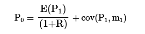
Price of asset with ITRS and rf

Cov() = risk premium

Interest rate short and long term

Rshort = R + inflation

RLong = R + inflation + theta

• theta = uncertainty about inflation

Taylor’s Rule

Break Even Inflation Rate

• Yield on non-inflation index bond - yield on inflation index bond

• inflation + theta

• yield nominal bond - yield ZCB

Required Rate of Return for Credit Risky Bond

Discount Rate for Equities

discount rate for commercial real estate

• R + π + θ + γ

  • γ = additional risk premium for credit risk = credit spread

• discount rate for equity = R + π + θ + γ + κ

  • κ = additional risk premium relative to risky debt for an investment in equities

  • λ = equity risk premium = γ + κ

• discount rate for commercial real estate = R + π + θ + γ + κ + φ

  • κ = risk premium for uncertainty about terminal value of property (similar to the equity risk premium)

  • φ = risk premium for illiquidity

Active Return /w Active Weights

• Active Return

  • E(R_A) = E(R_P) − E(R_B)

• Active Weight

  • E(R_A) = ΣΔw_iE(R_i)

    • Δw_i = active weight of security i = w_Pi  ​− ​w_Bi

Active Return Decomposition

Return in Benchmark + Active Return in Portfolio

Risk Adjusted Active Return (alpha)

Rp - β * Rb

• R_P is the portfolio's return.

• R_B is the benchmark's return.

• β is the portfolio's beta relative to the benchmark

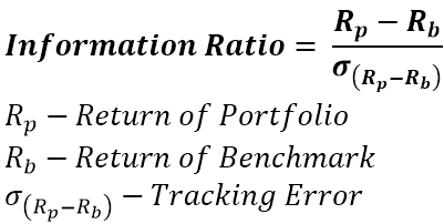
Sharpe and Information Ratio

SR = Rp - Rf / stdp

market neutral funds SR = IR

Optimal Active Risk

SR w/ optimal active risk & Portfolio total risk

Information Coefficient

Corr(forecasted, realized returns)

• measurement of skill

IC	Meaning
+1	Perfect forecasting skill
0	No skill (forecasts unrelated to outcomes)
−1	Forecasts perfectly wrong (consistently backwards)

Transfer Coefficient

TC = ρ(μ_i/σ_i,Δw_iσ_i).

Corr(Active Weight, Optimal Weight)

• For an unconstrained active portfolio, the active weights will be equal to the optimal weights and TC = 1.

• For a constrained portfolio (e.g., constraints on short positions or active risk), TC may be less than 1.

Breath (BR)

number of independent active bets each year

• if a manager takes active positions in 10 securities each month, then BR = 10 × 12 = 120.

Grinold Rule

μᵢ = IC × σᵢ × Sᵢ

IC = skill, σᵢ = risk, Sᵢ = score of security (standardized, variance of 1)

mu is alpha

Expected active return (3 ways)

E(R_A) = Σ Δwᵢ μᵢ

Sum of weight differences × expected alphas

E(R_A) = TC × IC × √BR × σ_A

IR × σ_A

Optimal information ratio (unconstrained + constrained)

IR* = IC × √BR

Unconstrained portfolio

IR = TC × IC × √BR

TC = transfer coefficient

Optimal expected active return (unconstrained)

E(R_A)* = IC × √BR × σ_A

IR* × σ_A

Optimal active risk (constrained portfolio)

σ_A* = TC × (IR*/SR_B) × σ_B	IR* = unconstrained IR; SR_B = benchmark Sharpe ratio

Sharpe ratio of constrained portfolio

SR_PC = √(SR_B² + TC² × IR*²)

Benchmark Sharpe squared plus TC² × IR*²

Expected Active return given IC, and TC

Share from Skill

Expected active return given IC	E(R_A | IC) = TC × IC × √BR × σ_A	Same as the constrained expected active return from the first table
TC²	TC² = share of active return from skill	Fraction of active return explained by the forecasts
Noise	1 − TC² = noise	Fraction of active return unrelated to skill

IC from market timing

IC = 2(% correct) − 1

If correct 50% of the time, IC = 0

'COMBINED ACTIVE RISK

AKA FULL ACTIVE RISK

Std. dev. of return differences (R_x − R_y)

$$\sigma_{C} = \sqrt{\sigma_{x}^{2} - 2\,\sigma_{x}\,\sigma_{y}\,r_{x,y} + \sigma_{y}^{2}}$$

Current Active Risk not optimal

Active annualized risk and return

square root of the sum of active weights squared times the active volatility squared for each security

Tilts

Risk Budget Active / Full Active Risk

breadth adjustment for correlated decisions

maximum spread

Total Cost / Round Trip trading cost

total cost = round-trip trading cost + management fees

round-trip trading cost = round-trip commission + spread

spread = bid ask spread

APT Equation

E(R_P) = R_F + β_P,1(λ₁) + β_P,2(λ₂) + ... + β_P,k(λ_k)

Macro 2 Factor Bond returns

R_i = E(R_i) + b_i1F_GDP + b_i2F_QS + ε_i

F are surprises

Fundamental Equity Model

R_i = a_i + b_i1F_P/E + b_i2F_SIZE + ε_i

Factor Active Return

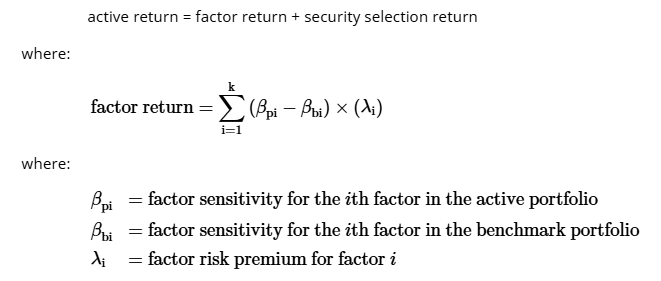
Active Risk / TE

Active risk = tracking error = σ_{(RP – RB)}

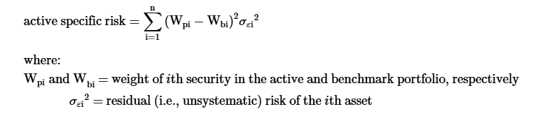
active SPECIFIC risk

active factor risk + active specific risk

stde = risk NOT EXPLAINED by the model

Cahart Model

E(R) = R_F + β₁RMRF + β₂SMB + β₃HML + β₄WML

where:   

• E(R) = expected return      

• RF = risk-free rate of return

• RMRF = return on value-weighted equity index − the risk-free rate   

• SMB = average return on small cap stocks − average return on large cap stocks   

• HML = average return on high book-to-market stocks − average return on low book-to-market stocks  

• WML = average returns on past winners − average returns on past losers

Portfolio std

VaR

[E(r ) - alpha *(port std)](-1)

annualized mean/ std

mean * n

std * sqrt(n)

change in call price

$$\Delta V \approx \text{delta}\,\Delta P + \frac{1}{2}\,\text{gamma}\,(\Delta P)^{2} + \text{vega}\,\Delta\sigma$$

one two tail table crit value 10%, 5%, 1%

Significance level (α)	One-tailed z	Two-tailed z
10%	1.28	1.645 (≈1.65)
5%	1.645	1.96
1%	2.33	2.576