Midterm 2 - Statistics and Experimental Design

Qualitative and Discontinuous Data

Data that exists as 2 or more distinct categories with no intermediate forms

Quantitative and Continuous Data

Data that exists at more than 2 distinct categories/has intermediate forms

Central Limit Theorem

For continuous variables, if n is sufficiently large (i.e., ≥ 30), then the:

1. mean of the sample of measurements should approximate the mean of the entire population

2. distribution of measurements should approximate a normal distribution (i.e., cluster around the mean with no bias to the left or right)

Accordingly, when making measurements, it is often the case that the bigger the n, the better the scatter of points approximates a normal distribution.

Mean (x̄) Equation

x̄ = Σx (sum of values)/ n (sample size)

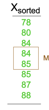
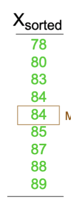
Median

The middle value (or average of the two middle values) in a set of sample

Mode

The value that appears most frequently in a data set

Law of Large Numbers

As one increases n, the parameters describing a sample (e.g. the mean) are less likely to be affected by random variation. This is because fluctuations in the data and outliers will cancel each other out.

One outlier can distort the mean when the n is small. The impact of the outlier is diminished as n increases → median is a measure of central tendency that is less vulnerable to outliers

Normal Distribution

Mean, median, and mode are roughly the same in this distribution.

The mean is a valid measure of central tendency only when this is the distribution (symmetrical and bell-shaped) and the mean, median and mode are roughly the same.

Bimodal Distribution

This type of distribution has two different means, but a roughly similar mean and median.

Distribution skewed to the right

Distribution where mode < median < mean.

Distribution skewed to the left

Distribution where mode > median > mean.

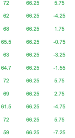
Residual Variation of the Mean

(Xi - x̄ )

Difference in each data value from the mean

Sum of Squares

SS = ∑(Xi - x̄ )²

Sum of all squared residuals from data set

Sample Variance (s²)

The calculated variance from a sample of a population

s² = SS/ (n - 1) ← penalized 1 degree of freedom when making an estimate about the population, rather than actually studying the entire population

When n is small, outliers dramatically distort estimates of variation

Standard Deviation (s or SD)

SD = √ s²

represents the magnitude variation and provides a measure of the “noise” in a given measurement

coefficient of variation (CV)

overcomes the problem with s² and s (which increase with size of the mean) by dividing s by the mean, yielding a measure of relative variation.

CV = (s/x̄) x 100

ex: one might want to know whether the weight of adult African Bush elephants is more variable than that of adult lab mice, without the s increasing with the mean.

confidence interval (CI)

directly illustrates whether two means differ significantly by the amount of standard deviations it differs from the mean by.

downside: bars are large and thus makes your data look noisy

95% CI = (z-score)(standard error) or 95% CI = mean ± t*SE

box-and-whisker plot

represents numerical data with the median, inter-quartiles and min-max values

this method of data presentation is often used to represent data that lack a normal distribution of scores

raw values

By presenting the responses of each experimental unit, this method of data presentation provides greater transparency

ex: the data in panels B-E could be represented accurately by the bar graph in panel A. However, the bar graph in panel A obscures the true nature of the data.

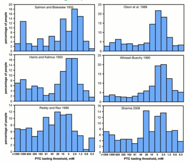
importance of non-normal distribution

Some measured variables never follow a normal distribution, even with large sample sizes. This may reflect something important, such as heterozygosity in a bimodal distribution.

A researcher measures the body mass of randomly selected adult mice from a large population. The population has a true mean body mass of 25 grams. According to the law of large numbers, what should happen as the researcher increases the sample size?

The sample mean will tend to become closer to the true population mean of 25 grams.

A researcher compares variation in body mass between two species of mammals. Species A has a mean body mass of 20 g and a standard deviation of 5 g, whereas Species B has a mean body mass of 100 g and a standard deviation of 10 g. Which statement best describes the difference in body mass variation between the two species?

 Species B has greater absolute variation in body mass, but Species A has greater variation relative to its mean.

Why are the residuals from the mean squared when calculating the sum of squares?

 

Squaring the residuals prevents positive and negative deviations from canceling one another.

A researcher measures the daily food intake of 20 mice. Most mice consume between 3 and 5 grams per day, but one mouse consumes 15 grams. Which statement best describes how this unusually high value affects the mean and median?

 The mean will be more strongly influenced by the unusually high value than the median.

Statistical Inference

focuses on making generalizations, predictions, or population-level conclusions from a smaller subset of subjects using statistical tests.

Experimental design

Focuses on how data are gathered, how treatments are applied, and how external noise/confounding factors are minimized before the experiment starts.

Yields objective criteria to determine whether an observed difference between sample means is reasonably consistent with the sampling variability under a null hypothesis.

Sample Means

Estimates of population means, which are subject to sampling variability.

Differences between these means can arise by chance, even when the population means are identical.

A larger observed difference does not necessarily constitute stronger evidence to reject the null hypothesis if variability is large.

True

Probability (p)

The likelihood that an event will occur, given all possible outcomes.

Used to identify unlikely events, outcomes, or responses.

Assumptions when calculating probability

• each time a die is thrown, all numbers occur with equal probability

• when multiple die are thrown, the results occur independently of one another

z-score

tells you how many standard deviations from the mean each data point falls

z = (Xi [individual data point] – population mean)/population SD (s)

Comparing Likelihood to a Large Population

1. Identify a test of interest

2. Administer the test

3. Compare outcome to the mean and SD of a large population of scores collected. The population mean and SD values would be considered the “true” mean and SD.

4. Convert each student’s IQ score (i.e., Xi) to a normalized z-score, using the z-score equation.

5. Based on the table for standard normal (z) distribution on the following page, values that fail to qualify would have scores < 1 SD.

z-distribution

• Helps to demonstrate which values are significantly different from the mean, or the values that are unlikely to occur from chance.

• The z distribution varies symmetrically around a mean of zero. The units along the x-axis reflect standard deviations (s) above and below zero.

• Can only be used when a reliable mean and SD of entire population are known.

Statistical Hypothesis Testing

Asks whether the observed data are compatible with a specified null hypothesis.

Null Hypothesis (H_o)

Hypothesis that predicts no effect or difference

In statistical testing, the goal is to determine whether or not you can reject it.

Alternative Hypothesis (H_A)

Hypothesis that predicts an effect or difference.

Test statistic

Quantifies how far the observed result departs from the null expectation relative to the sample’s variability

Proportional to: (observed effect - null effect)/SE

Null distribution

Describes how the test statistic would vary if the null hypothesis was true

p-value

The level of certainty an experimenter would require to be convinced that the observed difference is not due to chance alone.

If the chosen p-value = 0.05, then the experimenter believes that the outcome would occur 5 times by chance alone if repeated 100 times.

Quantifies how unusual the observed result is relative to the null model.

If a result passes the alpha level, the p-value must be unusual, and the event will occur more than 5 times if repeated 100 times (indicating that event did not occur by chance alone).

Decision threshold (alpha level)

A pre-specified criterion for rejecting the null hypothesis.

When N > 120, most scientists use 1.96 SD (95% confidence interval) above and below the mean as a decision level (alpha level = 0.05)

If a result passes the alpha level, the p-value must be unusual.

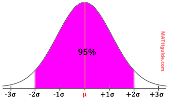
t-distribution

• Similar to a z-distribution, helps to demonstrate which values are significantly different from the mean, or the values that are unlikely to occur from chance.

• If the true mean and SD of a population is unknown, we have to use this distribution, with n-1 degrees of freedom.

• t-value determined by the critical values of t table

Testing the Null Hypothesis

Step 1. Calculate the standard error of the mean

Step 2. Determine the 95% confidence interval using the t-distribution

Step 3. Calculate the margin of error

Step 4. Calculate the 95% confidence interval

If the population mean falls outside of the 95% confidence interval found through your sample, you can reject the null hypothesis at the 0.05 alpha level.

Margin of Error

Margin of error = t*(SE)

Type 1 Error

• “Crying wolf”

• Rejecting the null hypothesis (stating that an event is significant) when it is not

• Reduce the risk: making this error by reducing the alpha level, causing us to expect a difference as large as (or larger than) the one obtained with the new alpha level (ex: 0.01 = 1/100). This lowers the threshold necessary to claim significance, reducing the risk of claiming significance falsely.

Type 2 Error

• Failing to detect the wolf

• Claiming that an event is not significant (accepting the null) when the event is significant.

• Reduce the risk: Design the study so that it has the power to reject the null that is actually false → reduce noise and bias, standardize procedures, increase sample size, create a larger effect size

• Large amounts of noise can obscure treatment effects

T-Test

A tool to determine if two means differ statistically, relative to their variability or noise.

Can only test 2 treatment values (control and treatment).

T-Value

Value that quantifies the difference between two means

Formula: t-value = explained variation/unexplained variation

Unpaired t-test

T-test used for between-subject designs — experimental units in each treatment level are independent

t = mean₁ - mean₂/pooled variance of both means (Sqrt[(s2p(1/n1 + 1/n2)])

If the observed t-value is > the critical t-value (found in the table of critical t-values), reject the H₀

Paired t-test

Used for within-subject designs - experimental units in each treatment level are not independent

t_paired = Mean_diff / SE_diff; the mean of the differences between both data points for one subject

Sample Variance of an Unpaired T-Test

s²_p= SS₁ - SS₂/n₁+n₂

Homoskedastic

Quality of a data set where each mean has a similar amount of variation (making sure you’re comparing apples to apples)

Assumptions of unpaired t-test

• Data are interval or ratio scales

• Randomly sampled

• Homoskedastic

• Distributions are normal

Assumptions of a paired t-test

• Data are interval or ratio scales

• Randomly sampled

• Each group displays a normal distribution

Two-tailed Hypothesis/T-Test

Hypothesis or t-test that is non-directional, has two rejection regions, and covers 2.5% of the (normal) curve’s graph

Example H₀: this drug will cause change to heart rate, relative to the baseline (mean)

One-Tailed Hypothesis/T-Test

Hypothesis/t-test that is directional, has only one rejection regions, and covers 5% of the curve’s area

Since the rejection threshold is closer to the mean, it is less stringent than a two-tailed hypothesis/t-test

Example H₀ : The drug will increase heart rate, relative to the baseline

Benefits of a One-Tailed T-Test

• Can determine significance easier than two-tailed t-test

• Demonstrates that you know your system and that you can make informed decisions

One-Sample T-test

Determines whether an unknown population mean differs significantly from a specific value, where the sample means of each population approximates the unknown population

Takes the mean_diff/SE_diff of each group, before comparing it to a critical t-value.

Assumptions of the one sample t-test

Data are interval or ratio scales

• Data were sampled randomly

• Underlying distributions are normally distributed (2)

Benefits of using > 2 t-tests

• Allows you to ask more sophisticated questions (ex: studying the degrees of a stimulus on an event)

• Allows you to study the functional relationship between a treatment and an event

One-Way Between Subjects ANOVA

A statistical method (test) that partitions variance into total variance, variance explained by treatment groups (between-subject), and variance not explained by treatment groups (within-group).

SS_total - SS_error = SS_treatment