Stats 100 midterm 3

Internal Validity

internal validity of a study depends on the similarity in the baseline characteristics between the control observations and the treatment observations. Basically, asking “can we trust that the casual factor actually caused the outcome in this study?”

• In order to have high internal validity, there must be a random component within a study.

• Studies with low internal validity would be case control and cohort control because they do not contain a random component.

• Studies with high internal validity would be matched pairs and block randomization because they contain random components.

Case control

a study in which individual control observations are each matched to individual “treatment” observations.

• case-control study starts with people who already had an outcome and compares them to people who do not have the outcome.

• It’s important to note that case-control studies typically have many pairs of matched observations

• The baseline characteristics within each match must be as similar as possible, but they do not have to be the same across matches.

Ex. We are looking at removing the attendance requirement for a class. We will use a case control study looking at the difference in grades for students who took a class with an attendance requirement and those who have not. We are looking at Asif and Yuli. Asif has taken the class with an attendance requirement, they had no prior experience in the class, no interest in the subject, no attention in class, and they spent 4 hours studying per week for the class (grade in class = 94). Yuli took the class without the attendance requirement, they had no prior experience, no interest in subject, no attention in class, and they spent 3 hours studying per week (grade in class = 93).

• Yuli and Asif are a good match for this study because they have very similar baseline characteristics. Asif is the control and Yuli is the treatment.

Cohort control

A study in which an entire group of control observations are matched to the group of treatment observations based on their baseline characteristics.

• We are considering an entire group at one time.

Ex. In the fall semester, the professor did not require attendance. Approximately 27% of students had prior experience in the subject. Approximately 18% of students expressed interest in the subject on Day 1 Survey. Approximately 59% of students were active participants in the class. On average, students spent 4.8 hours studying per week. The average grade was a 84%.

• We want to compare this group of students to the student in the spring semester of 2022. The spring semester of 2022 had an attendance requirement. There were 603 students, 28% had prior experience, 21% had interest in the class, 57% paid attention in the class, their average study hours per week was 5.0, and the average grade was 86%

• We are going to compare fall of 2023 with spring of 2022 because they have the most similar baseline characteristics.

• Fall of 2023 is the treatment group and spring of 2022 is the control group.

Random assignment

A strategy that utilizes a random process to determine which observations receive a treatment, and which serve as a control.

• Random assignment allows for higher internal validity because it reduces confounding variables, makes groups more comparable, and create less bias so more confident results.

Matched pairs

A strategy by which two observations are matched based on the important baseline characteristics, and then one observation in the pari is randomly assigned to the treatment group, while the other is randomly assigned to the control group.

• the researchers decide which observation gets exposed to the treatment and which does not.

Ex. We want to see if drinking tea has an effect on sleep. Anjali and Angel are matched on age. Anjali is randomly assigned to drink tea. Anjali’s and Angel’s sleep is measured.

Block randomization

A strategy by which an entire group of similar people are matched and blocked together, and then within each block, some are randomly assigned to the treatment group, while the others are randomly assigned to the control group.

• block randomization is by far the most common study design that statisticians and data scientist use to support making causal inferences.

Ex. we want to see how drinking tea affects sleep. Split everyone up by age groups, randomly assign some people to drink tea and some to not. Measure everyone’s sleep,

Sampling

The act of selecting observations from which to collect data.

Sample

The observations selected

population of interest

all observations that we are interested in studying or making a statment about.

inclusion criteria

The way in which statisticians define who or what is the population of interest is by specifying based on certain attributes.

parameters

The summary statistics for attributes based on an entire population of interest.

• the true number describing an entire population of interest.

generalization inference

The act of using a sample statistic to determine the value of a parameter.

estimate

The value we use as a stand-in for the parameter

external validity

the degree to which a sampling strategy supports making a generalization inference.

• the extent to which the observations in the sample are like the observations in the population of interest.

• a study can have higher external validity when its results can be generalized to a larger population or applied to real-world situations outside of the study.

• multistage has very high external validity because it uses random selection at multiple stages to create a representative sample of a large, diverse population. probability sampling has high external validity because participants are randomly selected, giving members of the population a known chance of being included.

• volunteer sampling, quotas, and survey incentives have low external validity because there can be bias because anyone can answer and people who do answer might have different characteristics from people who don’t volunteer.

representatives

The external validity of a sample depends on the extent to which the observations in the sample are like the observation in the population of interest, in terms of important underlying baseline characteristics. This is also known as the samples representativeness.

volunteer sampling

Sampling strategy in which you make a survey or study available to some or all respondents who meet the inclusion criteria.

probability sampling

A sampling strategy in which all eligible observations are assigned a non-zero probability to be included in the sample (every observation has a chance at being selected), and then some observations are selected using a random process.

quota sampling

A sampling strategy in which you have specific quotas (limits) for specific strata (similar groups in the population of interest) of respondents within the population of interest.

Ex. applying quota sampling to the study on Illinois farms, we might still spread the link as before but additionally apply a quota of three farms per country.

• In this case, each stratum is one county, and in essence we conduct a volunteer sampling with a fixed sample size within each county.

multi-stage probability sampling

Statisticians create complex sampling strategies that often include multiple stages and levels.

• The sample is selected in stages, with random sampling used at each stage.

Ex. We want to do a study involving all US adults. However, we cannot select all 250 million adults in the US to participate in the study. So, we can first start randomly selecting some of the states in the US. Every state has a chance of being selected. Next, we can randomly select some counties from each state we selected. Finally, we can randomly select some adults from each of the countries we selected, at last arriving at a sample of adults living in the US.

social exchange theory

Posits that in exchange for giving their data, respondents should get something in return.

survey incentive

The act of offering something in return for a respondent providing their data.

non-response

When a respondent selected for the sample chooses not to respond to the survey, either to specific questions or to the entirety of the survey.

• creates a problem in terms of the representativeness of the sample, especially in probability samples.

Posterior probability distribution

A special type of distribution that specifies how likely different potential values of a parameter are given the sampling strategy, data, and estimate that was collected.

Ex. What is the median salary in 2022 of all Americans over the age of 25 who have earned a bachelor’s degree? Our population of interest includes all Americans over the age of 25 who earned a bachelor’s degree which is almost 18 million people. In 2022, as part of the American community survey, the us census bureau recruited a nationally representative sample of all Americans over the age of 25 who have earned a bachelor’s degree by using a complex, multistage probability sampling strategy, and obtained information about each sampled persons salary. The sample median from this sample is approximately $64,911. How can we incorporate estimation error into our generalization inference?

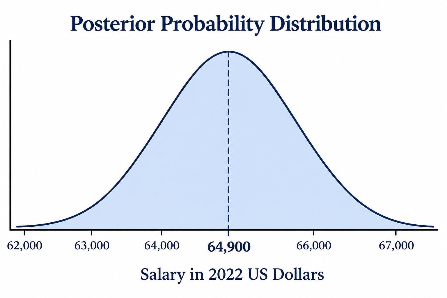
point estimate

the point estimate is our estimate of the population parameter, without incorporating “ish”-ness.

• a single # calculated from a sample that we use to estimate an unknown population parameter.

interval estimate

instead of using a single number as an estimate, we can use the entire middle 95% of the posterior distribution to provide an entire range of numbers as our estimate - this is called an interval estimate.

• a range of numbers used to estimate an unknown population parameter.

• values inside the interval estimate are values we think could probability be the true value. Values outside the interval estimate are values we think are probably not the true value.

To find the interval estimate lower limit we would subtract the point estimate form the margin of error. To find the interval estimate upper limit we would add the point estimate form the margin of error.

Margin of error

Inorder to find the margin of error we would do 2 times the estimation error.

Ex. the estimation error for the median salary of Americans over 25 with a Bachelor’s degree is equal to $149. Using this information, along with the point estimate of $64,911, we can construct an interval estimate using the equations. So the margin of error would be $298. The interval estimate would be [64,613, 65,209]

• the interval estimate is also the middle 95%

Bias

any systematic manner in which the data that has been collected has fundamental problem that will prevent the statistical methods from producing a correct estimate.

• common sources of bias are measurement bias, sample bias, and casual bias.

Measurement bias

Any bias in the data due to problems in the measurement process.

ex. if a researcher is interested in weighing several sodium crystals, but the scale has been calibrated incorrectly such that the readings are all 4 grams higher than it should have been, then each of the measurements for each of the observational values will also be too high.

Sample bias

Any bias in the data due to problem in the representativeness of a sample.

• especially important to consider when the purpose of an analysis is to make generalizations from the data to a population of interest.

• mainly about generalization inferences and external validity.

• if there is high external validity there is little sample bias.

Casual bias

Any bias in the data due to differences between the controls and observations in the treatment group.

• especially important to consider when the goal of a study is to make causal inferences and estimates of an average treatment effect

• has to do mainly with casual inferences and internal validity

• if there is high internal validity there is less causal bias.

Estimate’s precision

How much uncertainty we have, and therefore how much room for error we give, when we make an estimate of a parameter.

• the precision of an estimate is how narrow an interval estimate we can create based on the data (margin of error)

Evidence-based testing

Statistical testing that begins with data, creates a posterior distribution for a parameter, and subsequently evaluates hypothesis by comparing them to the posterior distribution.

• If we are using evidence-based testing, we would place the data in a posterior distribution. then consider the height of the hypothesis on the curve.

• in the picture example we see that 65,000 is very high on the curve meaning that it is likely the parameter

hypothesis-based testing

Statistical testing that begins with a hypothesis, creates a probability distribution based on that hypothesis and the estimation error, and subsequently evaluate estimates from the data by comparing them to the probability distribution.

• if we are using hypothesis-based testing approach we would make the probability distribution with the hypothesis in place of the actual point estimate.

• We would find the interval estimate using the margin of error and hypothesis. Give the photo example, we can assume that the point estimate (sample median) would be around 64,700 and 65,300 (middle 95%)

• If the actual sample median is 64,911m we would say that it is inline with our expectations, because it falls inside the range of values.

null model

Represents your expectations for what the data will be

• for when you make a probability distribution using the hypothesis-based testing

p-value

probability of seeing something even further away from what was expected than the observed data.

• This is how statisticians quantify the extent to which the observed data is consistent with their expectations.

• above 0.10 means there is consistency between expectations and actual data

• below 0.02 means inconsistency between expectations and actual data.

• in-between 0.10 and 0.02 means inconclusive results.

Regression

A method that is based on keeping the distance from all the points to the lines as small as possible (on a scatter plot)

• use to determine model coefficients model fitting

Prediction error

how far off the model’s prediction was from the real result

• to find the best line to match the data on a scatterplot we need to consider the distance between each point and the line, or the prediction error.

• for a single observation

• but all observations will have error so we can put all of the error into its own observation distribution or error distribution

Residual standard error

describes the typical prediction error

• find this by finding the standard deviation of prediction errors

• helps us to create prediction intervals for what we think the value of the response variable will be for a single observation if we know that observations values for the explanatory variables.

Prediction intervals

prediction intervals allow us to incorporate “ish”-ness into our model-based prediction.

• wider intervals mean more uncertainty

• narrower means less uncertainty

• to create a prediction interval, we multiply the residual standard error by 2. then we find the margin of error by multiplying 2 by the residual standard error. Lastly to get the limit we take the predicated value and add or subtract it by the margin of error.

• prediction intervals are for making a prediction for a single observation, and we use the residual standard error to quantify the uncertainty in our predictions

• only make prediction for single observations if there is very high internal and external validity

R squared

the percentage of variability in response variable that can be explained by the model

• provides judgement on the model’s usefulness’

• higher than 0.3 means that the model is very helpful in understanding the variability in the response variable, and the patterns the response variable has with the explanatory variable in the model.

z-scores

used to measure the difference between what we expect and what actually happened or between what we predicted and the actual result.

• we can directly compute the amount of prediction error for the observation

• z-scores below -2 or above +2 were values that are surprisingly far away from the predicted value