Ch9 forecasting error in prediciton

• Remember there are 3 tasks associated w/ correlation statistics 

1. Measure strength of relationship between two variabless by computing the correlation coefficient

2. Make optimal predictions of one variable from the other by finding the equation of the regression line 

3. Forecast the size the size of the a typical prediction error. 

   • This task is the subject of the present chapter

   • Once we understand the concept of forecasting the size of prediction errors, we will also be able to develop a more sophisticated system of interpreting a correlation than the crude on we presented in ch. 7

Forecasting prediction error:

• When we make predictions of one variable from another using the equation of the regression line, our predictions will be the best that we can make, but they will still not be perfectly accurate.

  • Therefore, it would be very useful to us to be able to know in advance how large a typical prediction error would be. 

    • As an ex: consider the set of data (from ch 7 and 8) in table 9-1 relating test scores to how long applicants stay on the joob at a fast food chain. Figure 9-1 shows the scattergram, of data from table 9-1, including the regression (predicition) line and prediction errors around the regression line

  • The prediction error for each subject (employee) is the difference between her actual time on the job (Y) and the time on the job predicted by using our regression equation (Y’). That is,

    • Prediction error = (Y-Y’) = (actual value of Y - predicted value of Y)

• graphically , the prediction error is the vertical distance from the actual value of Y( for a given subject) to the actual regression line. 

• These prediction errors for each of the five subjects in our ex are drawn on the scattergram in figure 9-1

image of figure 9-1

To calculate the standard deviation of these prediction erros we can use the old, familiar standard deviation formula from ch. 4… which is

(click on image to see the the old, familiar standard deviation formula from ch. 4 standard deviation formula)

To calculate the standard deviation of these prediction erros we can use the old, familiar standard deviation formula from ch. 4

• Since the “score” in this case is a prediction error, our formula becomes 

Standard deviation of prediction errors formula

Note, however, that the mean prediction error around the regression line will always be..

zero

• Note, however, that the mean prediction error around the regression line willa always be zero

• This is an inherent characteristic of a regression line, since it runs through the “middle” of the set of points

  • We can see and intuitively understand  this by looking at figure 9-1 

  • About half the points are above the regression line (and represent positive errors) and half are below (and represent negative errors). 

    • Thus these positive and negative differences between the points and the regression line will cancel each other and average out to be zero. So formula becomes= 

• So formula becomes= 

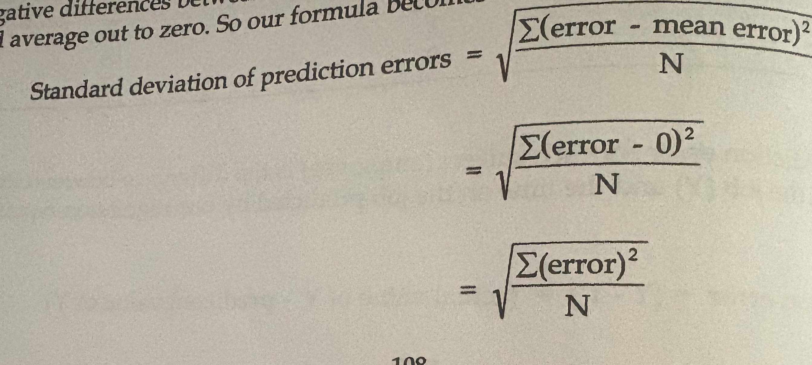
• Note, however, that the mean prediction error around the regression line willa always be zero

• This is an inherent characteristic of a regression line, since it runs through the “middle” of the set of points

  • We can see and intuitively understand 

  • this by looking at figure 9-1 

  • About half the points are above the regression line (and represent positive errors) and half are below (and represent negative errors). 

    • Thus these positive and negative differences between the points and the regression line will cancel each other and average out to be zero. So formula becomes

This quantity is a special kind of standard devatioin and is called the standard error of estimate.

• The notation S_est is commonly used to represent the standard error of estimate. So the fromula goes as follows

• S_{est =}  standard error of estimate

• = standard deviation of prediction errors around the regression line

• = (click on the image to see the rest of the formula)

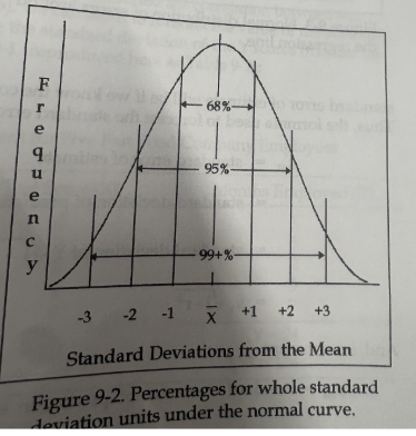
• Once we know the standard error of estimate we actually know quite a lot, because the standard error of estimate is a standard deviation and because prediction errors are normally distributed.

  • That is, now we can apply our knowledge of the normal curve and use our normal curve tables to tell us how many errors of any given size we would make if we used the regression equation to make predicitons of Y.

• Remember from ch 5 that in a normal distribution the number of cases falling within any given distance of the mean is easily found; we just have to express the distance in standard deviation (or z score) units

  • Figure 9-2 summarixes this info by just showing the percentages of scores falling within 1,2, or 3 standard deviations of the mean

image of figure 9-2

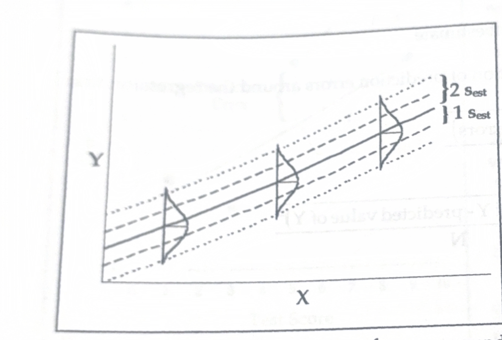
Our regression line can be thought of as a sliding mean and the standard error of estimate is the standard deviation of errors around it. This is illustrated in Figure 9-3.

• A critic might protest that this is not very useful because we must already have made our predictions and computed the prediction errors (Y - Y') before we can calculate their standard deviation. (Remember, we want to be able to forecast the size of the standard deviation of prediction errors). So this is somewhat like locking the barn after the horse has been stolen. 

• Fortunately, there is another way to calculate the standard error of estimate that does not require that we first make each prediction and then compute each prediction error.

  • That is, we can forecast what the standard errror of estimate will be if we know the correlation between the two variables. Thus the formula used to forecast the standard error of estimate is 

the formula used to forecast the standard error of estimate (click on the image to see formula)

How can we forecast what the standard errror of estimate will be

if we know the correlation between the two variables

formula used to forecast the standard error of estimate is 

fomula for forecast the standard error of estimate is 

The truly obstinate critic might still protest that our formula for forecasting the standard error of estimate from knowledge of the correlation still requires us to know ..

• the standard deviation of Y

  • However, this is not much of a problem because the standard deviation of Y (the criterion variable) is usually known, can be readily obtained from past data, or at the very least, can be estimated from the sample data in our study.

Computing the standard error of estimate:

• To illustrate the computation of the standard error of estimate, consider our example in which we want to predict how long employees will stay on the job in a fast food restaurant. Fast food restaurants have been around for many years; and this particular fast food restaurant has probably also been in operation for at least a few years. So we know from past experience how long employees tend to stay on the job?

• The standard error of estimate provides us with the answer to this question. Because we already (in ch 7) calculated the correlation between test score and months on the job (r=.76), we can use it to forecast the value of the standard error of estimate.

• First we calculate the standard deviation of the Y scores (months on the job) using the data table from table 9-1 (reproduces here as table 9-2) 

Table 9-2 Test scores and length of employment for five fast food company employees:

Employee	Test score (x)	Months employeed (y)
1	5	7
2	7	5
3	3	2
4	1	3
5	9	7 (sum symbol)Y=24 (sum symbol)Y2=136

computing the standard error of estimate

example:

Using our old raw score formula for the standard deviation (from Chapter Four), but using Y instead of X as the variable in the formula, we calculate the standard deviation as follows:

• As a check, we can make actual predictions,

• As a check, we can make actual predictions, calculate the prediction errors, and compute the standard deviation of these prediction errors.

•   For this example, we can use the equation for the regression line (which we computed in Chapter Eight) to make a prediction for every fast food employee in our study. Then we can compare each prediction (Y’) to that employee's actual length of employment (Y) to get each prediction error.

  • Finally, we can calculate the standard deviation of these prediction errors. It should be the same value as we forecasted (1.33). This check is shown below.

• Recall from ch 8 that our regression equation for this fast food company example data is

  • Y’= .55x + 2.05

  • or

  • predicted length of employment = .55(test score) + 2.05

• Using our example data in Table 9-2, we substitute each employee's test score for X in the regression equation to get a predicted number of months of employment (X) for each employee:

  • Y'employee 1 = 55(5) + 2.05 = 4.80

  •   Y'employee 2 = 55(7) + 2.05= 5.90

  • Y'employee  3 = 55(3) + 2.05 = 3.70

  • Y'employee 4 = 55(1) + 2.05 = 2.60

  • Y'employee  5= 55(9) +2.05 = 7.00
    
    
    

Now we compute our prediction errors (y-y’) and find the standard devaluation of these prediction errors (the standard error of estimate) as shown in the table below 

table 9-3 example

• Using our example data in Table 9-2, we substitute each employee's test score for X in the regression equation to get a predicted number of months of employment (X) for each employee:

  • Y'employee 1 = 55(5) + 2.05 = 4.80

  •   Y'employee 2 = 55(7) + 2.05= 5.90

  • Y'employee  3 = 55(3) + 2.05 = 3.70

  • Y'employee 4 = 55(1) + 2.05 = 2.60

  • Y'employee  5= 55(9) +2.05 = 7.00

Now we compute our prediction errors (y-y’) and find the standard devaluation of these prediction errors (the standard error of estimate) as shown in the table below in table 9-3

(click on image to see the example)

This value of the standard error of estimate (1.32) calculated directly from actual prediction errors is within rounding error of the value of the standard error of estimate (1.33) that we forecasted using our knowledge of the correlation. So our check indicates that our method of forecasting the standard error of estimate really does work (and it is easier than having to make actual predictions and calculate the prediction errors first)

example of table 9-3

Interpreting Correlations Revisited

(click on image attatched to see table 9-4, Best Guesses (the Mean) and Actual Months of Employment for Five Fast Food)

• In Chapter Seven we presented a table (Table 7-3) that provided rules of thumb for making rough interpretations of correlation coefficients of various sizes. Now, armed with an understanding of the standard error of estimate, we are in position to based on a comparison of prediction error and guessing error

• GUESSING ERROR  Assume that in our fast food company example we had no knowledge of X (the test scores) and therefore could only guess at Y (number of months the newly hired employees would remain on the job). It turns out that our best guessing strategy would be to always guess the mean of Y. The reason for this is that the sum of squares (and, hence, the standard deviation) around the mean is smaller than it would be around any other value. Table 9-4 shows our best guess (the mean) for each fast food employee in our example and the guessing error.

• Table 9-4: Best Guesses (the Mean) and Actual Months of Employment for Five Fast Food

• Note that when we guess the mean, the sum of the guessing errors will always be zero. So the average guessing error will zero and the sum of squares for guessing will be: (click on image attached to see)

• This is nothing other than the sum of the squared guessing errors, or deviations around the mean of Y.

  • So the standard deviation of our guessing errors (when we employ the best guessing strategy by always guessing the Y mean) will always be the plain old standard deviation of Y.

  • In Chapter Four we presented the deviation score formula for calculating the standard deviation. Now we use this deviation score formula in terms of Y (instead of X as we usually see it) to calculate the standard deviation of guessing:

• Standard deviation of guessing errors= standard deviation of Y when we use the best guessing strategy (always guessing the Y mean)

  • (click on image to see this worked out)

image of..

Standard deviation of guessing errors= standard deviation of Y when we use the best guessing strategy (always guessing the Y mean)

• (click on image to see this worked out)

Prediction errors versus guessing error.

• Now we can compare our overall prediction error with our overall guessing error.

• Remember that our measure of the overall prediction error is the standard error of estimate the standard deviation of the prediction errors), and our measure of the overall guessing error is the standard deviation of Y (the standard deviation of guessing errors).

 Remember that our measure of the overall prediction error is the..

 standard error of estimate the standard deviation of the prediction errors

our measure of the overall guessing error is the

standard deviation of Y (the standard deviation of guessing errors).

Prediction error versus guessing error.

• Now we can compare our overall prediction error with our overall guessing error. Remember that our measure of the overall prediction error is the standard error of estimate the standard deviation of the prediction errors), and our measure of the overall guessing error is the standard deviation of Y (the standard deviation of guessing errors).

• example:

• S_est= 

• S_y=

• S_est=  = standard error of estimate = standard deviation of prediction errors = 1.32

• and

•  S_y= standard deviation of Y= standard deviation of guessing errors 

• Notice that the standard deviation of our prediction errors around the regresssion line (the standard error of estimate) is less than the standard deviation 

What does S_est =

standard error of estimate = standard deviation of prediction errors

What does S_y =

standard deviation of Y= standard deviation of guessing errors 

• Notice that the standard deviation of our prediction errors around the regresssion line (the standard error of estimate) is less than the standard deviation 

  •  This tells us that when we use our regression equation (that is, when we use our knowledge of the relationship between X and Y predict Y, our errors in prediction will be smaller than the errors we would make if had to guess.

  • In fact, if a correlation exists between X and Y, it will always be true th the prediction errors will be smaller than the guessing errors. Furthermore, when the correlation between X and Y is stronger, the disparity between the size of the guess error and the size of the prediction error will be larger.

  • Now we can directly compare the prediction error to the guessing error for our fast food example by forming a ratio: 

Standard deviation of prediction errors / standard deviation of guessing errors =

standard error of estimate/standard deviation of Y =  

S_est / S_y=

1.32 / 2.04= .65

• Our ability to interpret the fast food correlation rests on this ratio. It tells us that our overall prediction error is only 65% as large as our overall error if we guess.

• Figure 9-4 shows a scattergram of both our prediction errors around the regression line and our guessing errors around the mean. In Figure 9-4 we can easily see that, overall, the prediction errors are smaller 

quantitative interpretation of correlation 

• We are now in a position to develop a sophisticated quantitative system of interpretation for the Pearson r correlation coefficient. We simply take the relationships, formulae, and definitions that we have coefficient. We simply take the relationships, formulae, and definitions that we have developed so far in this chapter and combine them, using a little bit of simple algebra and a dollop of logic.

• We begin with our formula for forecasting the standard error of estimate from our knowledge of the correlation:

(click on image attatched to see it worked out)

k =

coefficient of alienation 

• =proportion of guessing error remaining in our predictions =

  • square root of 1- r²

• However, often what we are interested in is not how much guessing error is left in our predictions but rather what proportion of guessing we are able to eliminate by making predictions using our regression equation.

  • Once we know the coefficient of alienation, it is easy to get this new information. We know that

  • the amount..

• Amount of error eliminated by making predictions =  total amount of guessing error - amount of guessing errror reminds in our predictions 

• Expressing this as a proportion of the total guessing error, we get 

  • Proportion of guessing errror eliminated by making predictions = 1 - proportion of guessing error remaining in our predictions 

  • Or

  • Proportion of guessing error eliminated by making predictions = 1 - coefficient of alienation  = 1 - K = 1 - (square root of) 1-r²

    • This quantity, which is also frequently used in the interpretation of correlations, is called the index of forecasting efficiency. The symbol for the index of forecasting efficiency is E. 

The symbol for the index of forecasting efficiency is, what…

E

E= index of forecasting efficiency = proportion of guessing error eliminated by making predictions = 1- k =

1- (square root of) 1 - r²

(click image to see this worked out)

E= index of forecasting efficiency = proportion of guessing error eliminated by making predictions = 1- k = 1- (square root of) 1 - r²

These two quantities (E and k) allow us to interpret the strength of correlations in terms if a standard deviation (of guessing errors).. what do they tell us

(K= coefficient of alienation, E= the index of forecasting efficiency)

• the proportion by which the standard deviation of guessing errors is reduced by making predictions (in the case of - the index of forecasting efficiency),

• or the proportion of the standard deviation of ressing errors still remaining in our predictions (in the case of k - the coefficient of alienation)

These two quantities (E and k) allow us to interpret the strength of correlations in terms if a standard deviation (of guessing errors).. what do they tell us

(click on image to see formulas)

• the proportion by which the standard deviation of guessing errors is reduced by making predictions (in the case of - the index of forecasting efficiency), or the proportion of the standard deviation of ressing errors still remaining in our predictions (in the case of k - the coefficient of alienation)

• However, sometimes we find it useful to interpret the strength of correlations in terms of a variance, rather than a standard deviation. To do this, we return to our basic standard error of estimate formula: s_est = s_y (square root of) 1- r²

• if we divide bothe sides of the equation by s_y we get….

• next is we square both sides of the equation we get….

• Looking at the left side of the equation since s_est, Is the standard deviation of prediction errors, then s_est²  is the variance of prediction errors.  similarly since  s_y Is the standard deviation of y, then  s²_y Is the variance of Y. Using these definitions our equation becomes….

• or, expressing this as a proportion we get

  • Proportion of variance of Y not accounted for by a knowledge of X= 1 - r² 

  • This is another quantity that is frequently used for interpreting correlation as the coefficient of non-determination. So we can summarize:

  • Coefficient of non-determination=

    • =Proportion of the variance of Y not accounted for by a knowledge of X

      •  = 1 - r²

(click on image to see this worked out)

These two quantities (E and k) allow us to interpret the strength of correlations in terms if a standard deviation (of guessing errors).. what do they tell us

The coefficient of non-determination provides useful information, but what we really want to know is what proportion of the variance of Y is accounted for if we know X. Now we can easily find this quantity:

• 
  

  • Proportion of the variance of Y accounted for by a knowledge of X = All of the variance of Y -  Proportion of the variance of Y not accounted for by a knowledge of X

• OR

  • Proportion of the variance of Y accounted for by a knowledge of X = 1 - (coefficient of non-determination)

• So

  • Proportion of the variance of Y  accounted for by a knowledge of X= 1-(1-r_²) 

• And by simple algebra: 

  • Proportion of the variance of Y accounted for by a knowledge of X= 1 - 1 + r² = r²

    • This quantity is called the coefficient of determination and is most frequently used quantity for interpreting correlations . To sumamrize, 

      • r² = coeffcient of determination = Proportion of the variance of Y accounted for by our knowledge of X

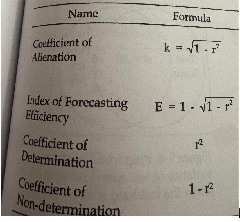
What is the Coefficient of alienation formula and what info is provided

• (click on image to see formula)

• Information provided 

  • Proportion of guessing error remaining when we make predictions bases on our knowledge of the relationship between X and Y

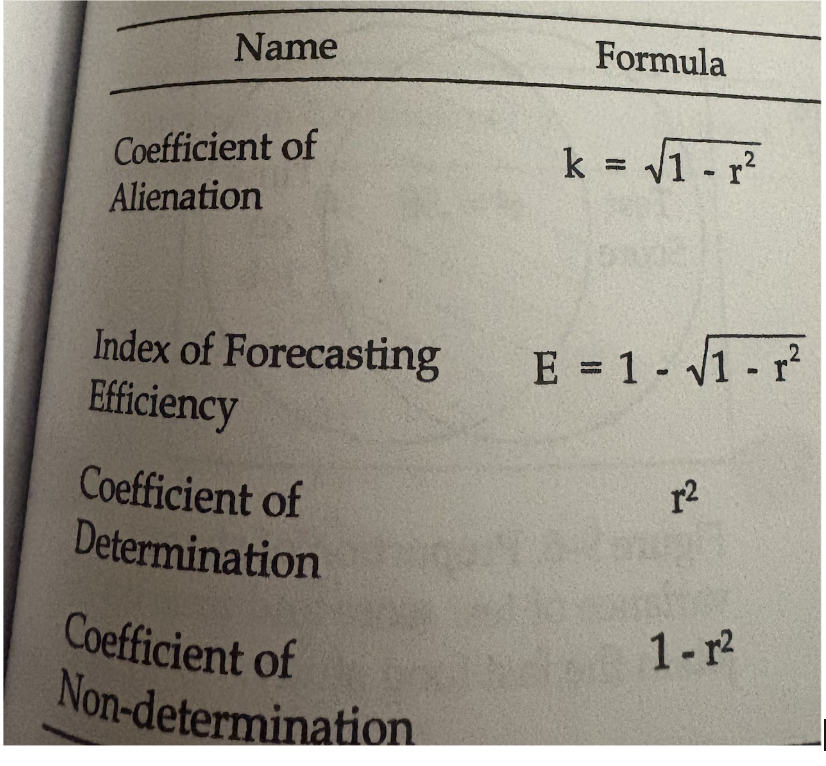
What is the Index of forecasting efficiency formulq, and what is the info provided

• (click on image to see formula)

• Information provided:

  • Proportion of guessing error eliminate by making preidictions, rather than guessing

What is the Coefficient of determination formula, and what is the info provided

(click on image to see formula)

Info provided: proportion of the variance of Y that is accounted for by a knowledge of Y

What is the Coefficient of non determination formula, and the info provided

• (click on image to see formula)

• Info provided

  • Proportion of the variance of Y that is not accounted for by a knowledge of x 

image of pages 121-122

pages 121-122

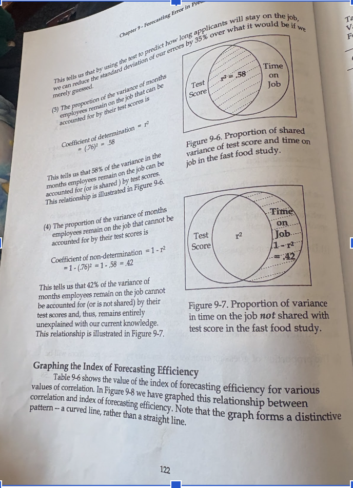
image pages 123 -124

pages 123-124