Advance Stats

Population

all members of a well-defined group.

–E.g. UTA students

*population is well defined such that one could determine specifically who all the members of the group are.

Parameter

a characteristic of a population.

–E.g. Students age, gender, type of car they drive, etc.

Sample

a subset of a population.

–E.g. Student in college of science, college of engineering, members of student senate, etc.

*Sample consists of some, but not all, of the members of the population

Statistic

a characteristic of a sample.

–E.g. Female psychology students at UTA

• Ex: how many employees in sample, the age, the average salary (sample statistics)

*Statistics of a sample do not have to be equal to the parameters of a population.

Descriptive statistics

techniques which allow us to tabulate, summarize, and depict a collection of data in an abbreviated fashion.

–E.g. graphs and tables instead of entire datasets.

*Descriptive statistics provide a summary of data usually in a table or a graph format so that we can understand the bigger picture.

Interferential statistics

techniques which allow us to employ inductive reasoning to infer the properties of an entire group of individuals (i.e., a population) from a small number of those individuals (i.e., a sample).

–E.g. sample of 5000 UTA students prefer beer over wine therefore UTA students prefer beer.

*allows us to collect data from a sample of individuals and then infer the properties of that sample back to the population of individuals. Logically speaking this is inductive reasoning because we go from specific to general.

Using sample stats to use logic to infer what the population parameters would be, based on the sample stats

-need representative sampling

-Different sampling methods

Better at picking the sample the better data, prediction and so on

Types of variables

Constants: what you are controlling in your study

-Doesn’t change within the study

-Variables: do change

-Categorical: stats students (something you can put in a category) aka qualitative

-Numerical: dichotomous (yes/no, true/false, two selections), continuous variables: scales, scores, the variable can take on any numerical value (ex: study gets a 50, another gets a 49.889

-Discrete (whole numbers, only take certain values, things we can count)

Numerical variable

quantitative variable

• either discrete or continuous  

Discrete variable

a numerical variable that arises from the counting process that can take on only certain values.

–E.g. # of children in a family, students in a class, etc.

• Variable that can only take on certain values (whole numbers)

  • Ex: number of children in a family can only take on certain values (no negative children or decimals of children, can’t have half a child) 

For example number of children in a family, you can’t have negative number of children or 1/3 of a child. Also it wouldn’t matter if we started counting from front of the class to the back or from left to right, we will end up with the same number of students in the class.

Continuous variable

a variable that can take on any value within a certain range, given a precise enough measurement instrument.

–E.g. weight, time, etc.

Continuous variable can take on any value within a certain range depending on the precision of the measuring instrument for example weight scale that measures up to 100^th value or a clock that measures passage of time down to picosecond!

Dichotomous variable

a variable that can take on only one of two values (a restricted case of a discrete variable).

–E.g.  Pass or Fail, Dead or Alive, etc.

• Ex: gender at birth (female or male), pass/fail, living/dead

  • Dichotomous variables have a special importance for binary logistic regression 

Variable

any characteristic of persons or things that is observed to take on different values.

–E.g. Annual salary in a particular neighborhood, types of careers students choose, beer preference, etc.

Constant

any characteristic of persons or things that is observed to take on only a single value.

–E.g. Career preference of women in STEM fields.

When designing a study, you can determine what is a constant. This part of the process is called delimiting, or narrowing the score of your study. For example, say you want to know what career path girls in STEM field are taking. You’ll be delimiting your study to girls, therefore gender would be a constant variable.

Categorical variable

qualitative variable

–E.g. political affiliation, religious affiliation, letter grade, etc.

Categorical variable is a qualitative variable that describes categories of a characteristic or attribute.

Measurement

•Measurement scale dictates what statistical procedures can be performed with the data.

These scales increase in complexity with nominal scale providing the least information and ratio scale providing the most information.

Nominal scale

Units are classified into categories so that all those in single category are equivalent with respect to the characteristics being measured 

• Qualitative/Categorical 

  • Could use numbers but they would have no numerical value, would simply be a way of identifying 

    • Ex: Jersey numbers, number 20 is a person not a number 

      • Categories are mutually exclusive = Can only belong to one group

      • Other examples: hair color, eye color, neighborhood, sex, ethnic background, religious affiliation, political party affiliation, type of life insurance owned (e.g., term, whole life), blood type, psychological clinical diagnosis, Social Security number, and type of headache medication prescribed

–Statistics of nominal scale variable are simple: frequencies that occur within each of the categories.

•Brown eyes – 10

•Blue eyes – 9

•Purple eyes – 0

Ordinal scale

Determined by the relative size or position of individuals or objects with respect to the characteristic being measured 

• 
  

• Qualitative (sometimes quantitative) 

• Ranking order

  • Ex: class ranking based on gpa 

  • However equal differences between the ranks do not imply equal distance in terms of the characteristic being measures 

    • First and second could have a different distance from scoring than we think 

      • Consists of two mathematical properties: equality vs inequality, if two individuals/objects are unequal then we can determine greater than or less than 

      • Tied rankings (when two are the same, take the average, example two individuals with a 3.8 gpa would be ranked 2.5 both instead of 2 and 3 while the follow person behind is 4th)  

–Ordinal scale cannot tell us how much greater than or less than because of unequal intervals.

–Tied and Untied ranks.

Interval scale

Where units can be ordered and equal differences between the values do imply equal distance in terms of the characteristic being measured 

• Order and distance relationships are meaningful, however there is no zero point 

  • Ex: temperature (the temperature can go below zero, therefore zero is not a stopping point)

  • Equal distance (meaning temp can be equal distanced, 60 degrees is 5 degrees higher than 55 degrees, like 20 is 5 more than 15, however we can not say that 60 is twice as much as 30 degrees as there is no true zero value 

    • No True Ratios 

      • Equality vs inequality 

      • Greater than or less than if unequal 

      • Equal intervals 

Ratio scale

Ratio scale has all of the properties of the interval scale, plus an absolute zero point exist 

• True ratios exist due to the addition of a true zero 

  • Rank‑ordered, equal intervals, absolute zero allows ratios to be formed

  • Ex: Speed in 100‑meter dash measured in seconds, height measured in inches, weight measured in pounds and ounces, age measured in months, distance driven, elapsed time measured in seconds, pulse rate, blood pressure, calorie consumption

- There is an absolute zero (there is a stopping point) ex: test scores (0 on a test meaning that student has a zero on the test)

  - ZERO actually means something

Model

•Statistical models developed from observed data should predict real-world situations (psychological, societal, biological or economic).

•The degree to which statistical model represents the collected data is known as the “fit” of the model.

–Good fit: accurately represents real world situations and can be used to make accurate predictions.

–Moderate fit: some similarities to reality but also some important differences.

–Poor fit: does not represent reality well at all and cannot be used to make any useful predictions.

•Behavioral and social sciences tend to use Linear models.

–E.g., ANOVA & Regression

Frequency distributions

•We might want answers to questions such as:

a.which score occurred most frequently?

b.which scores were the highest and lowest?

c.where do most of the scores tend to fall?

•These questions can be answered with a frequency distribution.

• Ungrouped: 

  • Raw scores: (X) set of scores in their original form that has not been altered or transformed in any way 

  • How many times was the score observed (frequency) 

    • Use when fewer than 15 or 20 intervals (w= 1) 

Grouped: 

• Either minimal frequencies per score of larger number of unique scores (more than 20) than use 

Real limits and intervals

In order to cover or include any score that might occur, we need to use intervals rather than actual scores.

• Each interval actually covers a range of scores, with each interval having a midpoint, an upper real limit, and a lower real limit. 

• From the previous slide, consider the score or interval of 18.  This score actually represents the midpoint of that particular interval. 

Ex: someone getting a 18.25 instead of a solid 18 

• Upper real limit: halfway between midpoint of the interval under consideration and the midpoint of the next larger interval 

  • Ex: Midpoint 18, the next larger interval would be 19, therefore the upper real limit would be 18.5 

• Lower real limit: halfway between midpoint and next smaller interval 

  • Ex: 17 midpoint, next lower 16, therefore lower real limit would be 16.5 

• Width: difference between the upper and lower real limits of an interval (w= URL-LRL) 

  • Ex: w = 18.5-17.5 = 1.0 (then all intervals have he same interval width of 1.0) 

How do you determine what the proper interval width should be?

Interval width:
→ Number of scores included in each interval (e.g., 10–19 = width of 10)

Ungrouped:
→ Many frequencies per score + <15–20 unique scores
→ List each score separately

Grouped:
→ Few frequencies per score (1–2) OR >20 unique scores
→ Combine scores into intervals

Choosing interval width:
→ Pick a width that results in ≤15–20 intervals
→ Example: 1–100 → width of 5 = 20 intervals

Frequency distributions:
→ Can be used with any measurement scale (nominal, ordinal, interval, ratio)

Cumulative frequency distributions

Number of cumulative frequencies for a particular interval is the number of scores contained in that interval and all the smaller intervals 

• Ordinal but cannot be used with nominal 

Adding the total

The number of cumulative frequencies for a particular interval is the number of scores contained in that interval and all of the intervals below.

•Take the frequency column and accumulate/add upward.

•As a check, the cf in the highest interval should be equal to n.

Can be used with ordinal, interval, or ratio measurement scales.

Relative frequency distributions

Percentage of scores contained in an interval, also known as proportion or percentage 

• Take sample size into consideration allowing us to make statements about the number of individuals in an interval relative to the total sample (5/20 can say 20%)

Tell us not the raw score but what percentage achieved that score (making them into percentages/ decimals)

Frequency/ total number of students

Ex: people who scored 12 is 1 student, 1/25 = .04 or 4% got a score of 12

-All add up to 1 or 100%

-Looking at the proportions

•Takes sample sizes into account allowing us to make statements about the number of individuals in an interval relative to the total sample.

•Can be used with any measurement scale.

Cumulative relative frequency distributions

Percentage of scores in that interval and smaller 

• How many are HERE + everything BELOW?

  • And you calculate it by simply adding downward:

    • .04 → .04 + .04 = .08 → .08 + .08 = .16 → etc.

  • The final CRF should equal 1.00 (100%), because by the time you reach the highest score, you've accumulated everyone.

•Cumulative relative frequency distributions are used for ordinal, interval, or ratio measurement scales.

Bar Graph

•Bar graph of eye color data

•Bar graphs can be used with nominal measurement scales

Separated, each bar represents category itself, x and y

Histogram

•Histogram of statistics quiz score data

•An ungrouped histogram is represented here

•Histograms can be used with ordinal, interval, and ratio measurement scales

Doesn’t work with nominal, when talking about historgram the x is continuous, looking at the shape you can estimate the frequency

Frequency polygons

•Frequency polygon of statistics quiz score data

•Point at midpoint

•Frequency polygons can be used with ordinal, interval, and ratio measurement scales

Cumulative frequency polygons

•Cumulative frequency polygon of statistics quiz score data

•Point at upper real limit

•Cumulative frequency polygon can be used with ordinal, interval, and ratio measurement scales

• Involves plotting along y axis, points should be plotted at the upper real limit of each interval, the polygon cannot be closed on the right hand side 

Adding all the scores up, frequency we can see who got what at what point, cumulative always goes up

Shapes of frequency distributions

A.) Normal

Mean=median=mode

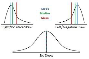
B.Positively skewed

•Mode<median<mean

b.) Right tailed, more lower scores towards the lower end

c.Negatively skewed

Mean<Median<mode

Scores bringing the mean towards the right

Percentiles

Percentile: score below which a certain percentage of the distribution lies 

Because percentiles are actual scores, they are continuous values, and can take on any value of those possible.

• Percentile Formula: Pi =LRL+(f(i%)(n)−cf )(w)

  • What each part means:

    • LRL = Lower Real Limit of the interval

    • i% = Percentile wanted (as a decimal)

    • n = Total number of scores

    • cf = Cumulative frequency below the interval

    • f = Frequency of the interval

    • w = Width of the interval

      • Example: Finding the 25th Percentile (P₂₅)

        • i% = .25

        • n = 25

        • cf = 5

        • f = 5

        • w = 1

        • LRL = 12.5

          • P25 =12.5+(5(.25)(25)−5 )(1) P25 =13.125

Quartiles

•Quartiles are special cases of percentiles where we divide the distribution into four equal groups (i.e., 25% in each).  Thus,

•Q₁ = P₂₅

•Q₂ = P₅₀

•Q₃ = P₇₅

• Can be used to determine if positive or negative skewed 

  • Compare the two distances:

    • Q3 − Q2 = spread of the upper half

    • Q2 − Q1 = spread of the lower half

  • If:

    • Q3 − Q2 > Q2 − Q1 → Positive skew
      → More spread out at the high end

    • Q3 − Q2 < Q2 − Q1 → Negative skew
      → More spread out at the low end

    • Q3 − Q2 = Q2 − Q1 → Symmetric
      → Equal spread on both sides

Percentile ranks

Percentage of a distribution of scores that falls below (or is less than) a certain score 

• Ex: scores falling below 150 score for GRE = 50% so therefore 50% of people score less than 150 on the GRE 

  • Formula: PR(Pi )= ncf+(wf(Pi −LRL) ) (100%)

    • What you need:

  • cf = cumulative frequency below the interval

  • f = frequency of the interval

  • Pi = score you're finding the rank for

  • LRL = lower real limit

  • w = interval width

  • n = total number of scores

    • Example: PR of 17

      • PR(17)= 255+(15(17−16.5) ) (100) PR(17)=22%

•Percentile ranks are basically the other side of the coin of percentiles. 

•Percentile ranks are percentages, while percentiles are scores.

•Computation of percentiles identifies a specific score, and you start with the score to determine the score’s percentile rank. 

Box-and-whisker plots

•Box-and-whisker plot of statistics quiz score data

•AKA "boxplot"

• Box (displays 50% of distribution scores) 

  • Black line = median (Q2)

  • Bottom edge represents 25th percentile (Q1) 

  • Top 75th (Q3) 

    • Scores that fall beyond the end of whiskers are outliers due to their extremeness

Summation notation

•Taking the sum of a set of scores is utilized quite often in statistics.

∑1_(i=1)^n▒X_i

•X = variable

•X_i = the score for variable X for a particular individual or object i

•i = serves to identify one individual or object from another

•Σ = the sum of

•i = 1 is the lower limit or beginning of the summation 

Central tendency

•Mean: “average,” is calculated by summing up all the values in a dataset and dividing by the number of values. Represents the balance point of the distribution and is sensitive to outliers.

•Median: is the middle value when the data is arranged in ascending or descending order. Its value separates the lower half of the data from the upper half. Less affected by extreme values and is useful with skewed distributions.

•Mode: value that appears most frequently in a dataset.

• Mode = nominal data 

• Median and mode = ordinal data 

• All three (median, mode, mean) = interval and ratio 

Mode

The mode is defined as that value in a distribution of scores that occurs most frequently.

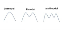
•Bimodal distributions can occur.

•Some people report both modes, while others average the two modes if they are adjacent.

•If they are not adjacent, do not average them.

•The mode is determined in the same way whether you are talking about a population parameter or a sample statistic.

One central point in the data, mode could be multiple (highest frequency), there could be a bimodal, when modes are closer, some people will take the average, but its not really recommended (list all modes instead)

General characteristics:

•simple to obtain (+): value that appears most frequently in a dataset.

•does not always have a unique value (−): can have more than one mode.

•not a function of all of the scores (−): less affected by outliers compared to mean.

•can be used with any type of measurement scale:

•Most often used with categorical or discrete data.

•Can be used with continuous data by grouping data into intervals and finding the interval with the highest frequency.

Median

The score which divides a distribution of scores into two equal parts 

• 1/2 of the scores fall below median, 1/2 fall above

Central point that divides the distribution in half, odd numbers (untied) the center value you can count from both ends towards the middle, even numbers (untied) take the two middle numbers and find the average of those score (n/2), any scale but nominal (no categories)

General characteristics:

a.not influenced by extreme scores (outliers) (+)

b.not a function of all of the scores (−)

c.always has a unique value (+)

d.can be used with any type of measurement scale except nominal

Mean

Average/ sum of all the scores divided by the number of scores (function of all the numbers)

• Population mean 

  • μ=N∑Xi/N

    • μ = population mean (average)

    • ΣXᵢ = add up all the scores

    • N = total number of scores in the population

• Sample Mean 

  • Same thing as pop but instead of mew (μ) its X (line above aka X bar) 

• Characteristics: mean is a function of every score, is influenced by extreme scores, mean always has unique value, mean is easy to deal with mathematically, only appropriate for interval and ratio measurement scales 

General characteristics:

a.function of every score (+)

b.influenced by extreme scores (−): outliers effect mean value.

c.always has a unique value (+)

d.easy to deal with mathematically; most stable of the measures of central tendency (+)

e.only appropriate for interval and ratio measurement scales

Measures of dispersion

•Another method for summarizing a set of scores is to construct an index or value that can be used to describe the amount of variability among the scores. 

•That is, do the scores tend to fall fairly close to the central tendency measure or are the scores fairly well spread out? 

•These indices are known as the measures of dispersion (or variability). 

•Here we consider the most popular such measures:

•range, (highest and lowest values [0,100] range 100-0 = 100

•H spread,

•variance, and

standard deviation

Range:

Influenced by extreme scores, function of two scores only, range is unstable from sample to sample, data tat are ordinal, interval or ratio in measurement scale 

Exclusive range

difference between the largest and smallest scores in a collection of scores 

• (ER) = Xmax - Xmin

  • Fails to account for the width of intervals being used 

    • Exclusive ranges mean the scores can be excluded from this range

      • Ex: a shoe costing 59.45 dollars and 75.65, the width being 1 so ranges would fall between 59.5-75.5 (the actual cost of the shoes fall outside that range, meaning they are excluded)

Values between two values, not including those values ex: what is the range between 10 and 70 , 70-10=60 (exclusive) did not include the value of 70 or 10, but instead the value between

Inclusive range

difference between the upper real limit of the interval containing the largest score and the lower real limit of the internal containing the smallest score in a collection of scores 

• Inclusive range adds the extra space at both ends so all possible scores are included

  • R=URL(Xmax )−LRL(Xmin )

    • URL = Upper Real Limit of the highest score

    • LRL = Lower Real Limit of the lowest score

Inclusive: values that could include decimals, 70.5-9.5 = 61 (including the ranges) width of more than one its different

H spread

•H spread relies on the difference between the third and first quartiles, Q₃ – Q₁.

•This is also known as the interquartile range.

•H measures the range of the middle 50% of the distribution.

•The larger the value, the greater is the spread in the middle of the distribution.

• Characteristics

  • Unaffected by extreme scores, not a function of every score, not very stable from sample to sample, appropriate for all sales of measurement except nominal  

Deviation scores

•The difference between a particular raw score and the mean of the collection of scores (i.e., population or sample).

•Summing the deviation scores will always equal 0.

•Thus, any measure involving simple deviation scores will be useless in that the sum of the deviation scores will always be zero, regardless of the spread of scores.

•Because it sums to zero, it is rarely used in statistics.

• The positive deviation scores will exactly offset the negative deviation scores. Thus, any measure involving simple deviation scores will be useless in that the sum of the deviation scores will always be zero, regardless of the spread of the scores

Population variance

is a statistical measure that quantifies the spread or dispersion of data points in a population. It provides insight into how much individual data points deviate from the population mean.

• Variance = average of the squared deviations from the mean.

variance

Definitional formula: conceptually the variance is a measure of the area of a distribution and more specifically the spread of the distribution from the mean 

• The more spread out the scores the more area or speak the distribution takes up and the larger the variance 

  • Also thought of as the average distance from the mean 

Sample variance

is a statistical measure that estimates the spread or dispersion of data points in a sample. It serves the same purpose as population variance but is used when you are working with a subset of data (sample) from a larger population

Standard deviation

deviational measure in the original scale, can take the square root of the variance 

• Function of every score 

• Affected by extreme scores 

• Only appropriate for interval and ratio measurement scales 

• Quite useful for deriving other statistics 

• The mode and range share certain characteristics 

• Population standard deviation: positive square root of the population variance 

• Bias

  • Something is systematically off 

Outliers

Step one: find the quartiles 

• Q1: 25th 

• Q3: 75th 

Step two: calcite the interquartile range 

• IQR= Q3-Q1 

  • The IQR represents there spread of the middle 50% of scores 

Step 3: calucatre the outliers senses 

• Lower fence= Q1 - (1.5xIQR)

• Upper fence= Q3 + (1.5xIQR)

  • Example: Q1 (20), Q3 (40)

    • IQR = 40-20=20

    • Then calculator 1.5 x IQR 

      • 1.5(20)=30

    • Fences

      • Lower = 20-30=-10 

      • Higher = 40+30=70 

If any scores fall outside of the upper or lower fence then they are an outlier 

The normal distribution: Characteristics (family of distributions, unit normal distribution, area under the curve, points of inflection, asymptotic curve) 

Standard curve: allows us to make comparisons across two or more normal distributions as well as look at areas under the curve 

• Always symmetrical around the mean (each half if split is equal)

• Unimodal (one mode or one peak)

• Bell-shaped (normal curve) 

  • The mean, mode, median will always be equal to one another for any normal distribution 

    • No real single normal distribution but rather a family of curves 

    • Infinite number of normal curve, one for every distinct pair of values for the mean and variance 

      • Each curve has a different number but a general sense that if they are normal will all technique be equal 

  • Unit normal distribution: mean of 0 and variance (standard deviation) of 1

    • Aka standard unit normal distribution  

•mean = median = mode

Converting distribution into any standard distribution (z score)

we can convert any normal distribution to a unit normal distribution through the use of the z score equation

• this transformation is done by moving the curve along the X axis until it is centered at the mean of 0 (by subtracting out the original mean) and then by stretching or compressing the distribution until it has a variance of 1

Converting any distribution into any standard distribution (z score)

• Take raw score converting (standardizing it)

  • Take raw score – mean/ sd = z score

    • Ex: sd 15

      • 85 (score)- 100(mean)/15 (sd) = -1

        • Z score = -1

•this allows us to make the same interpretation about any individual’s score on any variable

•this also allows us to make comparisons between two different individuals, or across two different variables

Area

The percentage or amount of space of a distribution, either above a certain score, below a certain score, or between two different scores

• Area under the curve 

  • Can we determine the area above any value, the area below any value, or the area between any two values under the curve 

    • Area under the curve representing 100%, we look at chunks of that data and determine what falls within the data, above, or below, even between

Z score interpretations

What you want	Formula
Below positive z	Use table value
Above positive z	1−table value
Below negative z	1−table value of positive Z
Above negative z	Use table value of positive z

Finding the area between values: find the z-score for each score and then subtract

Standard scores

Z score: z = (X-u(mean)/o (standard deviation)

• Divide the deviation from the mean (numerator) by the standard deviation (denominator) the value derived indicates how many deviations above or below the mean a unit score falls 

  • 1 deviation, 2 deviation, 3 deviations  

    • 
      

    • Values of z only range from 0 to 4.0

      • Reasons for this, values about 4.0 are rather unlikely, as the area under that portion of the verve is negligible (less than .003%), second the values below 0 (negative zero scores) are not really necessarily present in the table, as the normal distribution is symmetric around the mean of 0

    • P(z): the area below the respective value of z, aka the area between the value of z and the most extreme left-hand portion of the curve 

  • Any normal distributed variable, regardless of the mean and variance, can be converted into a unit normally distributed variable 

  • Standardizing a Normal Distribution (z-score)

• Any normally distributed variable can be converted into a standard normal distribution.

• The standard normal distribution always has:

  • Mean = 0

  • Variance = 1

    • We do this by converting the original scores into z-scores.

    • The shape of the distribution stays the same; only the values on the x-axis change.

Z scores (comparing two different scores)

z_i=((X_i-μ))/σ

z_(cognitive ability)=((75-60))/15=1.0

 

z_motivation=((60-40))/10=2.0

Changing the mean changes the sd

Standardization is comparing two datas that cant be compared with raw scores but instead looking at the SD can help determine which relationship is stronger or weaker or if there is no difference

Cog ability is one standard deviation above mean

Motivation is two SD above mean

Z score

Characteristics of z scores:

a.provides comparable distributions

b.takes into account the entire distribution of raw scores

c.can evaluate an individual’s performance relative to the scores in the distribution

d.negative (e.g., −1) and decimal values (e.g., 1.5) occur, thus other types of standardized scores have been developed (next slide)

• Why is this useful?
  It lets us compare scores from different variables/distributions using the same scale.

  • Example: z = +1.00 → the person is 1 standard deviation above the mean

    • z = −1.00 → 1 standard deviation below the mean

    • z = 0 → exactly at the mean

  • Basically: z-scores put everyone on the same scale so we can interpret scores the same way.

• This allows for comparisons between two different cases across two different variables 

  • Standardizing a variable, it is only the values on the x axis that change, the shape of the distribution remain the same 

Skewness (lack of symmetry)

Negatively Skewed (left)

Mode > Median > Mean

Positively Skewed (right)

Mode < Median < Mean

• Skewness: extent to which a distribution of scores deviates from perfect symmetry 

  • Important because perfect distributions rarely occur with actual sample data 

    • Asymmetrical: 

    • Negatively skewed: skewed to the left, occur when most of the scores are toward the high end of the distribution and only few scores are towards lower end 

      • mode>median>mean

    • Positive skewed: skewed to the right, occur when most of the scores are towards the low end of the distribution and few scores are towards the high end 

      • Mode<median<mean

      • 
        

a.range of skewness values is approximately from –2 to +2

• Or -2 (S.E. of skewness) to 2(S.E. of skewness)

  • Standard error

perfectly symmetrical distributions have a skewness value of 0

Measuring skewness

take z score for each individual (square it), sum all N individuals, dived by number of N 

• (a) a perfectly symmetrical distribution has a skewness value of 0, 

• (c) negatively skewed distributions have negative skewness values, and (d) positively skewed distributions have positive skewness values.

  • Rarely find a distribution that isn’t skewed, never really any perfect ones 

    • Guide to skewness: 

      • +/- 2.0 relatively normal 

      • Skewness values outside the range of plus or minus two errors suggest a distribution that is non normal 

Kurtosis (peakedness)

Kurtosis (peakness) range -2 to + 2

• Leptokurtic (Data is being compressed)

• Platykurtic (data is spread out more)

• Mesokurtic (normal)

• Also defined as peakedness

  • Leptokurtic (very peaked) 

  • Platykurtic (relatively flat)

  • Mesokurtic (normal distribution) 

    • Finding kurtosis: take z score for each unit (4th power), sum all N individuals, divide by the number of individuals N, then subtract 3 

      • Range from neg to pos infinity, kurtosis can be computed on variables that are interval or ratio scales  

Characteristics of kurtosis measure

a.perfectly mesokurtic distributions have a kurtosis value of 0

• a.Close to zero is okay

• b.Gets closer to one its still okay

• c.2 then there is a problem

b.platykurtic distributions have negative kurtosis values

c.leptokurtic distributions have positive kurtosis values

distributions

Normality Check Using Skewness & Kurtosis

• Expected value for Skewness = 0

• Expected value for Kurtosis = 0

• Calculate cutoff:

±2(SE)\pm 2(\text{SE})±2(SE)

• If Skewness/Kurtosis is within ±2(SE) → ✅ Approximately Normal

• If Skewness/Kurtosis is outside ±2(SE) → ⚠ Potentially Nonnormal

Example:

• Kurtosis = -1.299

• SE = 0.833

• Cutoff = ±2(0.833) = ±1.666

Since -1.299 is between -1.666 and 1.666, the distribution is normal.

Shapiro-Wilk sig. test

greater than 0.05 then the data is normally distributed.

If it is below 0.05 then data deviates from normal distribution.

Transformations

Positive skew (right tail, skew > 0) → make big numbers smaller

• Square Root (√x)

• Log (log x)

• Reciprocal √

Negative skew (left tail, skew < 0) → make big numbers bigger

• Power (x², x³)

• Right tail → Reduce → √, Log

• Left tail → Lift → Power

Using probability we can determine

How much uncertainty exists in our sample statistics

how much confidence we place in our sample statistics

Probability terminology

event: an outcome of a trial

independence: an outcome of a trail has no effect on the outcome of subsequent trials

Dependence

mutually exclusive: an occurence of one event of the other event

Probability

p(A) = S/T 

• p(A) is the probability that outcome or event A will occur

• S = number of times that specific outcome or event A can occur 

• T = total number of outcomes or events possible 

  • A standard die has six possible outcomes: {1, 2, 3, 4, 5, 6}

    • The event A is rolling a 4.

    • There is only one way to roll a 4, so S = 1.

    • There are six possible outcomes altogether, so T = 6.

      • Substitute these values into the formula: P(4)=1/6

        • This is assuming the die is unbiased (the die is fair that the prob. Of obtaining any of the six outcomes is the same) 

Ranges from .00 - 1.00 (sum must be equal to one)

Prob of one means event must occur

Prob of zero mean event is certain to not occur

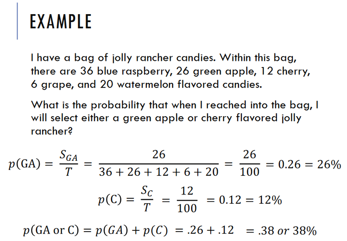
Additive Rule (Prob)

Given mutually exclusive events, the prob that one event or the other even will occur is the sum of the separate probs

Formula: p(A or B) = p(A) + p(B)

Multiplicative rule (Joint Prob)

Joint Probability: the prob of the co-occurrence of two or more events

• 
  

• Unconditional Prob: the prob of one event ignoring the occurrence or non-occurrence of some other event

Given independent events, the probability of the joint occurrence of the events is the product of the separate prob

p(A,B) = p(A)xp(B)

Conditional Probability

the prob that one event will occur given the occurrence of some other event.

• Dependent on an event

• ex: what is the prob of a person being a smoker, given they have lung cancer

p(smoker| lung cancer)

Sampling and estimation

•Since we rarely have population data, we rarely know what the population parameters are (e.g., population mean and variance).

•Thus, we almost always have sample data.  We would like to be able to generalize from our sample statistics back to the population parameters.

•Inferential statistics allow us to make an inference or generalization from a sample to the population.

If you know your entire population, then take 15 random, that’s the sample

Need multiple samples from multiple labs around the country, to verify a generalizable consensus for the entire population

• Larger the sample the better

Simple Random sampling

each observation has an equal chance of being selected

• Independence implies that each observation is selected without regard to any other observation sampled  

Simple Random with replacement

each observation is selected from the population and then put back

• Same number of population (meaning there is replacement each time) 

• Sample selected from population and observation is replaced back into the population

  • * Key is that each observation sampled is placed back into the population and could be selected again 

Simple Random without replacement

Once an observation is selected for a sample it is not replaced and cannot be selected a second time

• Once an observation is selected for inclusion in the sample, it is not replaced and cannot be selected a second time 

Types of sampling

Convenience sampling (volunteer)

• Example: A professor stands outside the library and surveys the first 50 students who walk by.

Systematic sampling (ex: every 10th / there is a pattern) 

• Example: A grocery store surveys every 10th customer who enters the store.

  
  

Cluster sampling (sample groups of observation include all members of the selected clusters) 

• Example: A school district randomly selects 5 classrooms and surveys every student in those classrooms.

  
  

Stratified sampling (sampling within subgroups to ensure adequate representation of each subgroup)

• Example: A university wants student opinions. They randomly sample:

  • 50 freshmen

  • 50 sophomores

  • 50 juniors

  • 50 seniors

Multistage sampling (stratify at one stage and randomly sample at another stage or randomly select clusters and then within clusters, randomly select individual units) 

• Example:

  1. Randomly select 10 high schools.

  2. Within each selected high school, randomly select 20 students.

Sampling distribution of the mean

Point estimate: simply one value or point then getting multiple samples 

• Ex: data sample one, data sample two, and so on 

Sampling distribution of the mean: collection of sample means, frequency distribution of sample means 

• The sampling distribution of the mean is created by taking all possible samples of a specific size and calculating the mean for each sample. For the population values 1, 2, 3, 5, and 9, (for ex: (1,1), (1,2), (1,3)…(7,4) etc) the population mean is μX=4 When all possible samples of size n = 2, are taken with replacement, there are 5×5 = 25, possible samples. The mean of each sample is calculated using Xˉ=X1+X2, producing 25 sample means that range from 1 to 9. 

• These sample means form the sampling distribution of the mean. When the 25 sample means are averaged together, the result is μXˉ=4, which is equal to the population mean. This demonstrates an important property of the sample mean: it is an unbiased estimator of the population mean because the average of all possible sample means equals the true population mean  

Sampling error

the difference (or deviation) between a particular sample mean and the population mean, denoted as X ̅-μ_X

•Positive sampling error indicates sample mean is greater than population mean (overestimation of the population mean)

• zero error: a sample mean exactly equal to the pop. mean 

•Negative sampling error indicates sample mean is smaller than population mean (underestimation of the population mean)

-More you increase sample the less error you will have

• Want the sample error to be close to zero as possible (suggest that the sample reflects the population well)

Variance error of the mean

The variance of the sampling distribution of the mean, which provides a dispersion measure of the extent to which the sample means vary and will also provide some indication of the confidence we can place in a particular sample mean.

The variance of the sampling distribution of the mean

• Variance error of the mean: variance is based on the sample mean = using sample variance and dividing by sample size

• Provide a dispersion measure 

  • Increasing the size of sample the magnitude of the sampling error decreases 

    • As sample increase, we hone closer to the pop mean and have less and less sampling error 

Standard Error of the Mean

•Standard error of the mean (standard deviation of the mean)

•σ_X ̅ =σ_X/√n

•The population variance error of the mean and the population standard error of the mean can be estimated by the following, respectively:

•s_X ̅^2=(s_X^2)/n

•s_X ̅ =s_X/√n

SE of sample means = standard deviation / square root of n

Confidence Intervals

A statistical range with a specified probability that a given parameter lies within the range.

Interval estimate for population mean 

• Sense of how confident we are 

  • One deviation = 68% confidence and so on 

    • 90% CI: 1.645

    • 95% CI: 1.96

    • 99% CI: 2.5758

    • 
      

•Conceptually, this means that if we form (68)% confidence intervals for 100 sample means, then 68 of those 100 intervals would contain or include the population mean (it does not mean that there is a 68% probability of the interval containing the population mean—the interval either contains it or does not).

Central Limit Theorem

•As sample size n increases, the sampling distribution of the mean from a random sample more closely approximates a normal distribution.

•If the population distribution is normal, then the sampling distribution of the mean is also normal in shape.

•If the population distribution is not normal, then the sampling distribution of the mean becomes more nearly normal as sample size increases.

•See following examples…

•This will become quite useful later on in inferential statistics, in particular, when the assumption of normality is not satisfied.

As we increase the sample size the closer we get to a normal distribution