Microeconomics (ch 5-7)

for midterm #2

price elasticity of demand

how responsive consumers are to a change in price (always positive)

E_d= (percent change in quantity demanded)/(percent change in price)

elastic demand

(E_d>1) consumers are highly responsive to a change in price. A small increase could cause a sharp drop in sales, usually because there are other substitutes. (ex. water bottles, baby wipes)

inelastic demand

(E_d<1) consumers are insensitive to price changes. Consumers will still demand a lot despite an increases in price, usually because substitutes are difficult to find (ex. gas, special drugs, spices)

unit elastic demand

(E_d=1) Ex. shoes, cars, salons

Cross elasticity of demand

measure how a change in the price of good B affects demand for good A (signs matter). Determines whether something is a substitute or a complement

E_ab= (percent change in quantity demanded of product A)/(percent change in price of product B)

substitutes

(E_ab>0) in increase is price of B increases demand for A, but brand loyalty can affects (like cars for example).

(ex. chicken/turkey, AT&T/Verizon, Fiji/Dasani)

complements

(E_ab<0) an increase in price of B decreases demand for A (coffee/creamer, burgers/fries, sausage/hotdog bun)

income elasticity of demand

how responsive quantity demanded is to changes in consumer income. Sign determines whether something is a normal good, luxury good, or inferior good.

(E_y= (percent change in quantity demanded)/(percent change in income)

normal goods

(0 < E_y < 1) as income rises, demand increased. (ex. clothes, food, etc.)

luxury goods

(E_y >1)A type of normal good, as income rises, demand for the good sharply increases (ex. jewelry, fine dining)

inferior goods

(E_y < 0) as income rises, demand decreases, usually to choose higher-quality options (ex. instant noodles, budget motels, generic soda)

price elasticity of supply

measure responsiveness of quantity supplies to price changes (always positive)\

E_s= (percent change in quantity supplied)/(percent change in price)

Elastic: (E_s>1) usually mass produced elastic goods and digital goods

Inelastic: (E_s<1) usually crops, natural resources, mining

Unit elastic: (E_s=1)

Market periods explain the lag between the popularity of a good and when its inventory can be replaced (ex. crops have longer market periods because its harder to grow more crops fast)

Tax incidence and burden

refers to who bears the ultimate economic burden of a tax (depends on elasticity)

Types of taxes

Progressive taxes, flat taxes, regressive taxes, lump-sum tax (type of regressive tax that takes a fixed amount of money), and excise taxes (placed on a specific typed of good and is usually included in the price of a good because producers pay it)

Mid point formula

used to calculate the price elasticity between two points (always positive)

E_d= (%△Q)/(%△P)

(%△Q)= (Q₂ - Q₁)/ ( (Q₂ + Q₁) /2)

(%△P)= (P₂ - P₁)/ ( (P₂ + P₁) /2)

total revenue test

(TR = P * Q) (total units sold times price of each unit) total output depends on price changes and elasticity

Inelastic demand: price and total revenue move in the same direction. (price increase raises TR)

Elastic demand: price and revenue move oppositely. (price increase lowers TR)

Unit elastic: price changes don’t affect TR

Elasticity along a linear demand curve

Elastic in the upper left: TR keeps rising until equilibrium is reached. Inelastic in the lower right: TR starts falling after equilibrium.

Tax Burden Rules (demand elasticity)

• Inelastic demand shifts tax burden onto consumers. Because they are willing to pay more, produces can afford to raise prices to cover the tax.

• Elastic demand shifts tax burden onto producers. If producers raise prices too much to cover the tax, consumer will stop buying.

Tax Burden Rules (supply elasticity)

• Inelastic supply shifts tax burden onto producers. Producers can’t easily change production rates or shift resources, to accommodate a tax

• Elastic supply shifts tax burden onto consumers. Producers can easily produce more/less or use their resources elsewhere, leaving consumers to deal with the tax.

Deadweight loss

the loss of total welfare when market is not at equilibrium

The greater the elasticity, the greater the deadweight loss from (especially from a tax)

Determinants of Demand elasticity

• Substitutability: goods with many substitutes have elastic demand

• Proportion of income: goods representing a larger portion of a budget (ex. housing) are more elastics compared to smaller parts of budget (ex. salt)

• Luxuries vs. necessities: luxuries are elastic, necessities are more inelastic

• Time period: the longer time you have to adjust your consumption patterns, the more elastic; the less, the more inelastic.

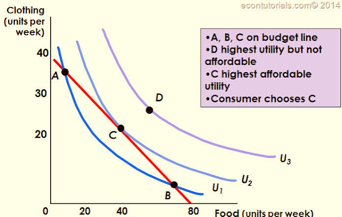
budget line

graph showing all the possible combinations of two goods a consumer can purchase with a fixed income and fixed prices

marginal utility analysis

how can you maximize consumer satisfaction?

Utility

a hypothetical measure of consumer satisfaction (measured in utils)

Total utility

cumulative satisfaction derived from consuming a specific total quantity of a good

marginal utility

the additional satisfaction gained from consuming one additional unit of a good

law of diminishing marginal utility

states that as we consume additional units, our marginal utility (the rate at which our satisfaction increases with each additional unit) begins to decline

utility maximizing rule

total utility is maximized where marginal utility per dollar is equal for all products

(MU_a / P_a) = (MU_b / P_b)

behavioral economics

integrates psychology into economic models to explain why some individuals make decisions that deviate from standard predictions

Budget line dynamics (price and income changes)

Price changes: a price change of one good pivots the budget line along that good’s axis (inward on the axis if price increases, outward if price decreases)

Income changes: an increase in income shift the line outward (parallel), a decrease shifts it inward.

Indifference curve

a curve displaying all combinations of two goods to which the consumer is indifferent (the receive the same level of satisfaction)

these curves have negative slopes and are bowed inward

optimal consumer choice

consumer satisfaction is maximized at the point where the highest achievable indifference curve touches the budget line

Five psychological factors influencing economic decisions

1. Sunk Cost Fallacy: allowing past, uncoverable costs influence you current choices rather than evaluating current marginal benefits (ex. going to a concert you paid for months ago rather than studying for an exam tomorrow)

2. Framing bias: being influenced by how choices/ prices are presented (ex. $2.99 vs $3.00 or BOGO free vs. 50% off entire purchase)

3. Overconfidence: overestimating future behavior vs capabilities (ex. buying an expensive gym membership that goes unused because you overestimated your ability to follow through

4. Overvaluing the present relative to the future: prioritizing immediate gratification over superior long-term benefits

5. Altruism: acting out of care for other without direct benefit (ex. generous tips)

Firm

an economic institution that transforms resources (inputs) into outputs. They must determine market need then decide what quantity of output to produce, how to produce it, and what inputs to use

Sole proprietorship

(most basic, easy to manage) a single owner supervises and manages the business and is subject to unlimited liability

partnerships

two or more owners sharing management and division of labor, subject to unlimited personal liability

corporation

owned by shareholders with less direct control from the owners. offers limited liability.

profit

total revenue (TR) minus total cost (TC)

total revenue

money a firm receives from the sales of its products

total cost

out-of-pocket expenses and opportunity costs

economic costs

explicit costs (expenses paid directly to another economic entity like wages, taxes, materials, etc) plus implicit costs

accounting profit

TR - explicit costs

economic profit

TR - (explicit + implicit)

normal profit

an economic profit of zero. sufficient to keep investors satisfied in the business over the long run

short run

a period over which at least one factor of production is fixed (ex. plant capacity)

long run

a time period long enough that all inputs can be adjusted and firms can enter/ exit the industry

Total product

total product produced by an amount of labor (used to change output in the short run where plant capacity is fixed). Experiences diminishing returns

marginal product

additional output produced by adding one more unit of labor

MP= (△Q/ △L)

average product

output per unit of labor. it’s subject to diminishing marginal returns.

(AP = Q/L)

Total costs

fixed costs (FC) + variable costs (VC)

variable examples: labor, materials

fixed examples: rent, insurance premiums

marginal costs

change in total cost from producing one additional unit. It’s curve passes through the minimum points of the AVC and ATC curves

MC= (ΔTC)/ (ΔQ)

average fixed cost

total fixed costs divided by output. Continually falls as output increases

AFC= (FC)/ Q

average variable cost

labor and materials expenses that goes into each unit. Is U-shaped, meaning it has initial increasing returns then diminishing returns.

AVC= (VC)/ Q

average total cost

provides a general measurement of productivity. Is U-shaped, meaning it has initial increasing returns (spreading effect) then diminishing returns.

ATC= (TC)/Q

aka

ATC= AFC + AVC

long run average total cost

shows the lowest unit cost for output levels produced in the long run when a firm can adjust its plant size. decreases as firm’s output increases

economies of scale

as a firm grows, its LRATC decreases because of specialization of labor and management and efficient capital use

constant returns to scale

as a firms output increases, LRATC remains constant (ex. fast food costs the same to produce almost anywhere)

diseconomies of scale

LRATC increases as a firm grows too big, usually because of management, coordination, and resource scarcity

economies of scope

by producing interdependent product lines, firms can produce them at lower costs. (ex. Unilever’s or Procter & Gamble’s household products