Econ Midterm 2

Topics: Taxes Externalities, Cost of Production, Perfect Competition, Monopoly, Public Goods & Consumer Choice

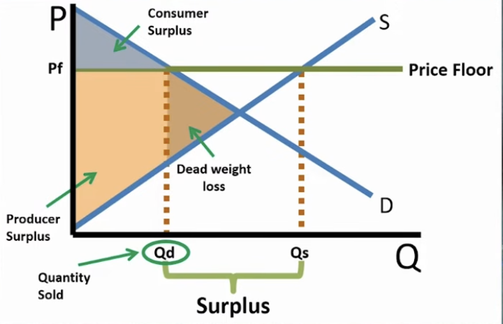
Price Floor

• legislated minimum (ex. minimum wage)

• market price is above equilibrium

• (price ceiling below equilibrium —> non-binding) price floor

Draw Price Floor (CS, PS, DWL, Surplus v. Shortage, etc)

Elasticity Impact on Price Floor

sInelastic S or D —> Small Surplus; Elastic S or D —> Large Surplus

Non-binding Price Floor

(price ceiling above equilbrium —> non-binding)

Price Ceiling

• legislated maximum

• market price is below equilibrium

• (price ceiling above equilibrium —> non-binding)

Elasticity Impact on Price Ceiling

Price Floor

• legislated minimum

• market price is above equilibrium

• (price ceiling below equilibrium —> non-binding)

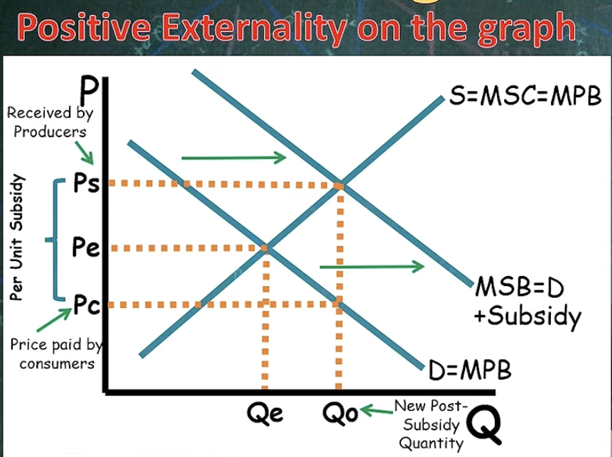
Subsidy (Draw Diagram with Ps Pe, Pb, S DWL curve and Subsidy curve

• payment to a producer or consumer for a product

• Subsidy Expenditure —> (Ps - Pb)Qs

Taxes

Ps —> anount sellers pay after tax

Pb —> amount buyers pay after tax

Tax Incidence

• who bears the burden of the tax (split)

Impact of Elasticity

• less elastic —> more tax (demand curve in this 1st image exanple)

• more elastic —> less tax (supply curve in this 1st image example)

Perfectly Elastic on Tax Incidence

No tax on either seller or buyer (demands which curve is perfectly elastic)

Perfectly Inelastic

Explicit Costs (chpt 14)

oppurtunity costs that require firms to pay out money

Implicit Costs (chpt 14)

• unobservable costs (skill, time, etc)

• forgone costs that don’t nesscarily require money

• a type of oppurtunity cost

Economic Profit (Equation) (chpt 14)

total revenue - (explicit costs + oppurtunity costs)

Accounting Profit (Equation) (chpt 14)

total revenue - explicit costs

fixed costs (chpt 14)

costs that do no vary with the quant. of output produced (FC)

Variable costs (chpt 14)

costs that vary with the quantity of output produced

Oppurtunity Costs (chpt 14)

• whatever must be given up to obtain some item

• implicit opportunity cost: the salary you gave up to run your own business. You make no payment, but it’s still a cost.

• Explicit oppurtunity cost: rent paid for the shop. Money leaves your pocket, and it could have been used

Equation to Maximize Profit (chpt 14)

Total Revenue - Total Cost (TR - TC)

Average Fixed Cost (chpt 14)

AFC = FC/Q

Average Variable Cost (chpt 14)

AVC = VC/Q

Average Total Cost (chpt 14)

ATC = TC/Q = AVC + AFC

Marginal Cost (chpt 14)

MC = ΔTC/ΔQ

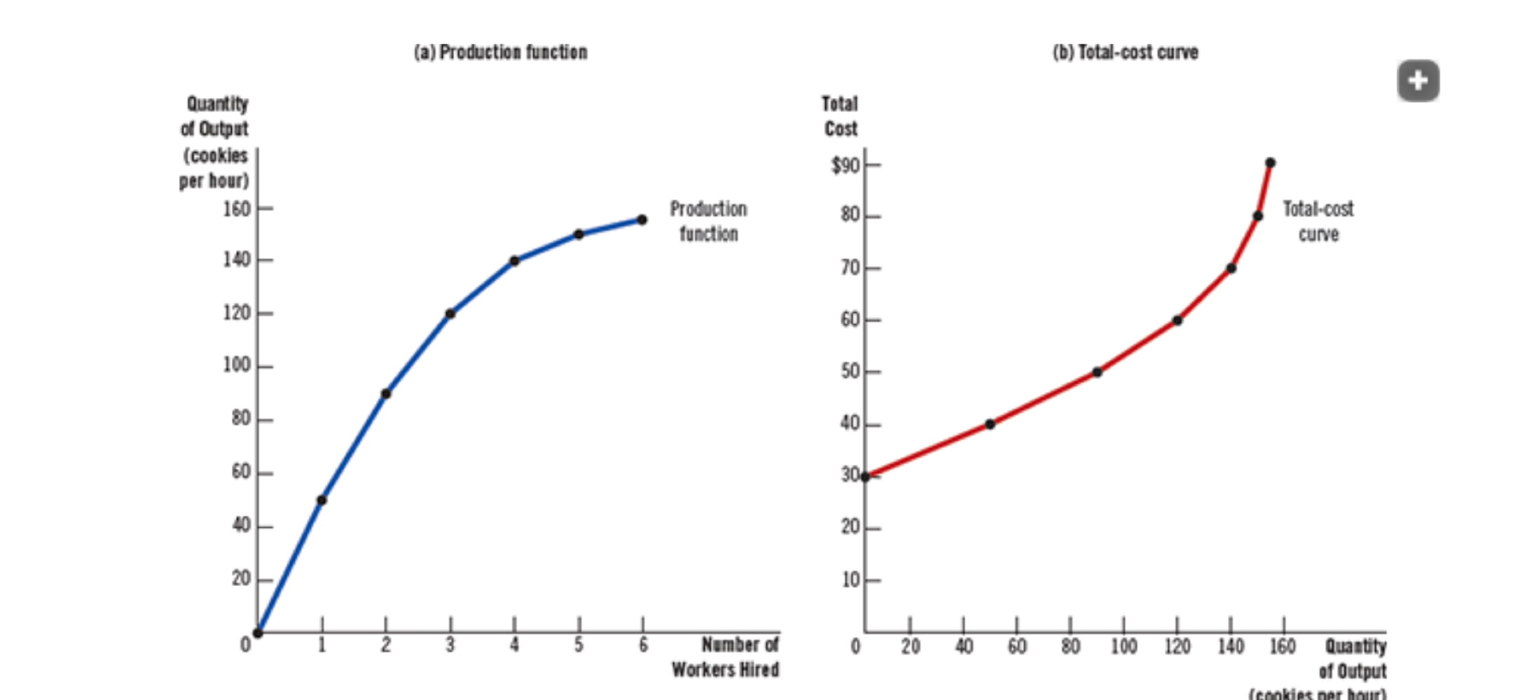
Total Cost

VC + FC

Graph of ATC and Marginal Cost (chpt 14)

• marginal cost rises with the quantity of output

• ATC falls first as output inc (MC < ATC)

• ATC rises as output continues to inc (MC > ATC)

• MC = ATC (at minimum of ATC curve —> efficent scale)

Efficent Scale (chpt 14)

the quantity of output that minimizes average total cost (ATC)

When is Profit Maximized (chpt 14)

MR = MC (which is equal to P)

Economies of Scale (chpt 14)

Long-run ATC falls as output rises

Diseconomies of Scale (chpt 14)

Long-run ATC rises as output rises (firm gets too big)

Constant returns to scale (chpt 14)

Long-run ATC stays the same as output rises (happens when firms can replicate ex. A coffee shop chain opens a second location identical to the first. Twice the workers, equipment and rent gives twice the coffee, so the cost per cup is unchanged.)

Marginal Revenue (chpt 14)

additional revenue earned from selling another unit

Sunk Costs (chpt 14)

cost that’s already been paid and can’t be recovered

Long run(chpt 14)

all costs are variable

Short run (chpt 14)

some costss are fixed (ex. wor

Diminishing Marginal Product (chpt 14)

The marginal product of an input falls as more of it is used (e.g., each added worker adds less output); this is why MC rises

Production Function (chpt 14)

“too many cooks in the kitchen”

if MC < AVC then AVC ___ and if MC > AVC, then AVC ___ (inc/dec) (chpt 14)

• dec, inc

• ex. Say your test average is 80 and you take one more test:

  • Score 60: below your average, so the average drops. (MC < AVC)

  • Score 95: above your average, so the average rises. (MC > AVC)

  • Score 80: the same as your average, so it doesn’t move. (AVC minimum)

• “ marginal pulls the average toward itself.”

If MC < ATC, then ATC & if MC > ATC, then ATC__ (chpt 14)

• dec, inc

• ex. Say your test average is 80 and you take one more test:

  • Score 60: below your average, so the average drops. (MC < AVC)

  • Score 95: above your average, so the average rises. (MC > AVC)

  • Score 80: the same as your average, so it doesn’t move. (AVC minimum)

• “ marginal pulls the average toward itself.”

Characteristics of Perfect Competition (chpt 15)

• many sellers + buyers

• identical products/services

• no barriers to entr

  y/exit

• price-takers

• MR = MC

Graph for Profit Maximizing (MC and ATC) (chpt 15)

Price > ACTC

Graph for Zero Economic Profit (MC and ATC) (chpt 15)

Graph for Profit Loss (MC and ATC) (chpt 15)

Steps for Finding Profit for Perfectly Competitive Firm (chpt 15)

1. Find the price.

2. Find the quantity where P = MC.

3. Find ATC at that quantity.

4. Calculate profit: Profit = (P − ATC) × Q

Profit Equation(chpt 15)

• Profit = (P − ATC) × Q or TR - TC

• P > ATC: positive profit

• P = ATC: zero profit.

• P < ATC: a loss

If P1 > ATC, firm woulld ___ and would attract ___ (chpt 15)

• stay in market

• attract entrance (until MR = MC)

If P < ATC and P>AVC, firm would…. (chpt 15)

• short run: stay operating ( sunk costs —> fixed costs

• long run: exit market

• firm is not profitable (but atleast covering AVC)

If P<ATC and P>AVC, firm would….(chpt 15)

short run: operate

long run: exit

If P<ATC and P<AVC, firm would….(chpt 15) b

short run: shut down

long run: exit

If P = AVC (chpt 15)

firm would be indiferrent to shut down —> revenue covers variable costs

Monopoly (chpt 16)

• one firm (usually gov gives exclusive right to produce a good/service)

• large barrier to entry

• price-maker

• firm can produce output at a lower cot that most firms (economies of scale)

Are Monopolies efficent? (chpt 16)

No because…

• create DWL if they don’t price discriminate (buyer aren’t not able to pay exactly their willingness to payz)

• while P = MR = MC (efficent quantitiy) in perfectly comp. firm in monopolies MR < P

Intuitive Example: Food truck example: why monopoly MR < P To sell more, the monopolist must cut the price for all customers. Revenue can even fall (100 sandwiches at $5 = $500; 110 at $4.50 = $495), so it stops where P > MC. The skipped customers (value > cost) are the deadweight loss.

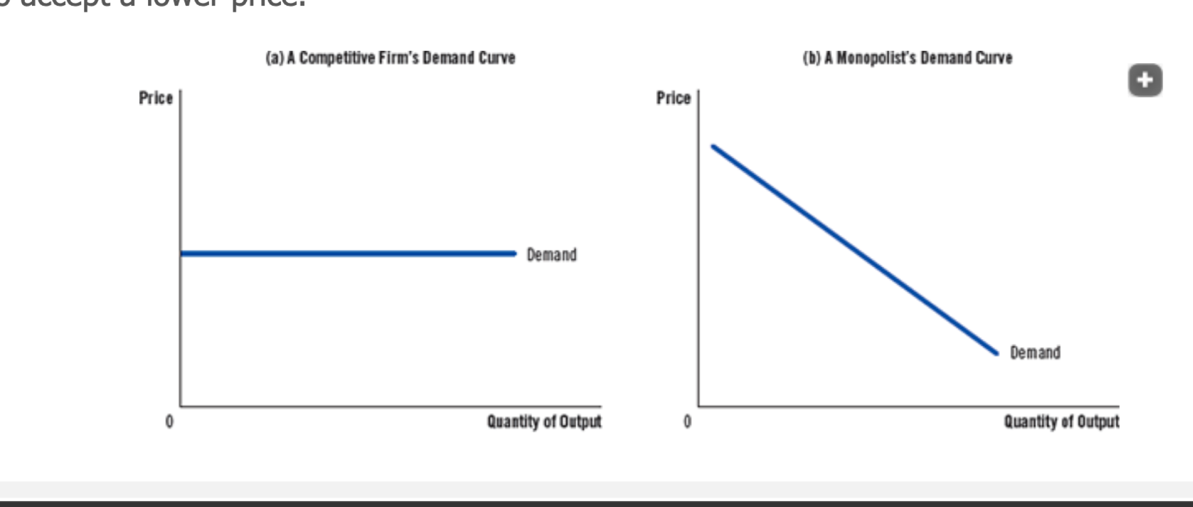
Competitive Markets Demand Curve (perceived for perfectly competitive market) (chpt 15)

• face horizontal demand curve because..

  • many sellers, each tiny

  • identical products

  • Free entry and exit

• therefore must accept market price…

  • , because the firm is so small that it can sell as much as it wants at P* but nothing if it charges more.

Monopoly Demand Curve (chpt 16)

Reading Monopoly Curves (chpt 16)

1. Find where MR = MC. Drop down to the quantity axis to get Qm.

2. Go up from Qm to the demand curve to find the monopoly price Pm.

3. Go down from Qm to the ATC curve. The rectangle between Pm and ATC (green), times Qm, is the profit: (P − ATC) × Q.

4. DWL: area between demand and MC, from Qm to where demand crosses MC (P = MC —> monopoly doesn’t produce efficent scale )

Practice Drawing Monopoly Graphs (ATC, MC, D, MR, Profit, DWL)

• constant MC, Constant MC = ATC, Increasing MC

(chpt 16)

Examples for Each

• Constant MC: the only cable company in a town. Laying cable is a huge fixed cost, but adding one more customer costs about the same each time. ATC falls as it adds customers.

• Constant MC = ATC: the only lemonade stand at an event, with no setup costs and a $2 cost per cup. Every cup costs $2, so ATC = MC = $2.

• Increasing MC: the only mine in a town. The first ore is easy to dig, but each extra ton is harder and more expensive.

Price Discrimination eliminates DWL and the surplus goes to…. (chpt 16 - monopolies)

Monopolies

Policymakers Response to Monopolies (chpt 16)

• anti-trust laws —> make industry more competitve

• price regulation that monopoly charges

• turn monopoly into government entreprise

Review Econ —> Monopoly Graph (chpt 16)

Monopoly vs Perfect Competition. What does this graph show?

1. Perfect competition (Pe, Qe): the market is at the point where demand crosses MC = S. That’s P = MC, the efficient outcome.

2. Monopoly (Pf, Qf): the monopolist follows MR = MC, which is where the MR curve crosses MC at Qf. Then it goes up to the demand curve to charge Pf. (Higher Prices, Lower Quantities

Natural Monopoly

• very high fixed costs + low marginal cost

ex. electrcity. water, cable internet

Positive Externality & Draw Graph (Chpt 10)

• uncompensated benefit to society

• underproduction

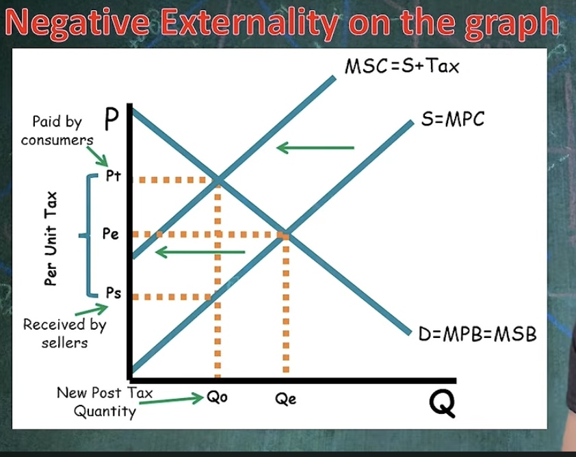
Negative Externality & Draw Graph (Chpt 10)

uncompensated cost to society

Correcting Negative Externalities (chpt 10)

Quantities restrictions

pollution permits

per-unit taxes

Per Unit Taxes on Negative Externalities

• with tax —> supply curve shift left

• per-unit tax —> compensates for externality

Corrrectlng Positive Externalities

• regulations

• public provision

• per-unit subsidies

•