Biostats Midterm (Ch. 1-8)

CH. 1

BIOSTATISTICS

Use of numbers to understand populations

The mathematical techniques used to organize data to test hypothesis

DATA

Organized numerical information

Questions = _______

Responses = ______

Variables

Cases

VARIABLE

a trait or a characteristic that can change values from case to case

(ex. eye color, income, age)

INDEPENDENT VARIABLE

the variable that causes something to happen

(ex. consuming calories)

DEPENDENT VARIABLE

the outcome or result variable

(ex. weight gained)

"ICE CREAM CAUSES DROWNING "

Causation VS Correlation

Not true, just a pattern and correlation that happen in the same direction

Both are caused by external variables (heat) and are not truly related to each other

UNIVARIATE vs BIVARIATE

univariate = 1 variable

bivariate = 2 or more variables

DESCRIPTIVE STATS vs INFERENTIAL STATS

DESCRIPTIVE

describes the distribution of a single variable (univariate) or the relationship between two or more variable (bivariate)

INFERENTIAL

involves using information from samples to make inferences about populations

DISCRETE VARIABLES

variable with a basic unit of measurement that cannot be subdivided

ex) number of siblings, number of people in a household, number of cars

CONTINUOUS VARIABLES

variable that has scores that can be subdivided infinitely

ex) time measured in minutes, seconds, milliseconds, test scores, length

NOMINAL VARIABLES

-variables that are descriptors and non-numerical

-cannot be ranked or ordered

-must be exhaustive, homogenous, and mutually exclusive (cannot appear more than once)

ex) colors, gender, race, religion, area code, etc

ORDINAL VARIABLES

-variables that have scores or categories that can be ranked from high to low

ex) opinion scales, social class, etc

LIMITATIONS: you can't measure the difference between ranks in precise units

INTERVAL RATIO VARIABLES

-scores that are actual numbers

-has a true zero point

-there is a set precision between 2 variables (fixed increments between them)

ex) age, income, GPA, number of children

CH. 2

PERCENTAGES

percentages = (f / N) x 100

f = frequency

N = number of cases in all categories

-easier to read and comprehend than raw frequencies

-standardize distributions to a base of 100

PROPORTIONS

proportion = f / N

-standardize results to a base of 1.00

-can convert percentages to proportions by dividing by 100 (ex. 37 / 100 = 0.37)

RATIOS

ratio = f1 / f2

f1 = number of cases in the first category

f2 = number of cases in the second category

ex. 1370 / 930 = 1.47

1370 Protestant families

930 Catholic families

*there are 1.47 Protestant families for every Catholic family (1.47:1 or could multiply by 100 = 147:100)

RATES

the # of ACTUAL occurrences divided by the # of ALL possible occurrences per some unit of time

ex) (number of death / total population) x 1000

100 - # of deaths / 7000 - total population x 1000

= 14.29 (for every 1000 people there were 14.29 deaths in 1998)

*rates can be multiplied by various powers of 10

PERCENTAGE CHANGE

tells you how much a variable has increased/decreased over a period of time

% change = (f2 - f1) / f1) x 100

f1 = first score, frequency or value

f2 = second score, frequency or value

ex) the death rate in 2005 was 50% higher than in 1995

FREQUENCY DISTRIBUTIONS

tables that report the number of cases in each category of a variable

exhaustive and mutually exclusive categories

CHAPTER 3

MEASURES OF CENTRAL TENDENCY

statistics that summarize a distribution of scores by reporting the most typical or representative value of the distribution

mode

median

mean

MODE

-the most common score, occurs most frequently

ex) set of scores: 58, 89, 92, 90, 58

*mode is 58 because it occurs twice

Used at NOMINAL (best), ordinal + interval levels of measurement

LIMITATIONS:

-some distributions have so many modes that is can be meaningless

-some distributions have no mode at all

MEDIAN (Md)

-the score of the case that is at the middle of a distribution

-must place cases in order from highest to lowest and locate the case that divides the distribution into two equal halves

*if number of cases is even, add the two middle cases and divide them by 2

ONLY used for ordinal (best) and interval variables

MEAN

-the arithmetic average of a distribution

-calculated by dividing the total sum of scores by the number of scores (N)

ex) administer a test to 5 clients. The number of correct responses were 2, 10, 15, 11, 9. Add the scores ( 47) and divide by number of scores (5) = 9.4 is the average score

*ONLY used for interval variables

CHARACTERISTICS OF THE MEAN

STRENGTHS

-uses all the available info from the variable

WEAKNESSES

-is affected by every score

-extreme high or low scores may skew the mean, making it misleading

-it's very sensitive when you only have a few scores

CH. 4

POSITIVE SKEW

-some very high scores

-pull the mean greater than the median

-mean pulled to the right = curve shifts to the right

-median stays in the center

MEAN AND MEDIAN IN THE SAME PLACE

not skewed

NEGATIVE SKEW

-some very low scores

-pull the mean lower than the median

-mean pulled the left = curve shifts to the left

MEASURES OF DISPERSION

-answers how do scores differ

-describes the variety, diversity, and heterogeneity

Ambulance Response Time example

-the greater clustering of scores around the mean indicate less dispersion and variation (shape of curve is more peaked) = more consistent choice

-the flatter curve shape indicates more dispersion/variety = less consistent choice

-had scores in the high and low ranges

RANGE

distance between the highest and lowest scores in a distribution

ex) 4 - 2.2 = 1.8

LIMITATIONS

-only based on 2 scores

-might exaggerate the amount of dispersion for most of the scores in the distribution (most distributions have some scores that are extremes)

-no info on variation of scores between highest and lowest

VARIANCE

s2 (deviations)

the squared deviations of the scores around the mean divided by N

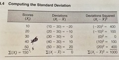
STANDARD DEVIATION

-the square root of the squared deviations of the scores around the mean, divided by N

-it uses ALL the scores in the distribution

-describes how far apart the scores are from each other

-increases in value as scores become more diverse (deviations large/spread out)

-decreases in value when the scores are more clustered around the mean (deviations small/less diverse)

s = standard deviation (deviations squared)

LIMITATIONS

-very suceptible to extreme scores in a small distribution because the mean gets pulled (SD gets bigger)

-can only calculate on INTERVAL variables

CHAPTER 5

STANDARD NORMAL CURVE

-unimodal (single peak)

-perfectly smooth and unskewed

-mode/median/mean are all the same value

-tail trails into infinity and never touches the abscissa

-theoretical, perfect model

-the distance under the curve when measured by SD always represent the same proportional area

Z SCORES

-standard way of measuring what percentage of the data falls where; always have the same values for their mean (0) and standard deviation (1)

-values that are not exact multiple of the SD must be converted to z scores

Xi = the score (72)

X bar = mean (65.59)

s = std dev (3.52)

z = (72 - 65.59) / 3.52

z = 1.82

NORMAL CURVE TABLE

-area between the score and the mean is exactly the same for a negative score as it is a positive score

a) Z score

b) area between mean and Z

c) area beyond Z

EMPIRICAL RULE

+/- 1s = 68.26% of the area

+/- 2s = 95.44% of the area

+/- 3s = 99.72% of the area

How many scores fall within 1 standard deviation (s) of the mean?

Mean = 144 lbs.

s = 33 lbs.

144 - 33 = 111 (16.2% under 111)

144 + 33 = 177 (8.1% above 177)

16.2% + 8.1% = 24.3%

100% - 24.3% = 76% of scores fall within 1s

Using z scores, what percentage of scores fall under 72 inches?

z = 1.82

a) 1.82 ------- b) 0.4656 (46.56%)

46.56 + 50 (other symmetrical half) = 96.56% of scores

Using z scores, what percentage of scores fall above 72 inches?

z = 1.82

46.56 + 50 (other symmetrical half) = 96.56% of scores

look in column c) for area above Z = 3.44%

(check that is equal 100 = 3.44 + 96.56)

Using z scores, what percentage of scores fall between 72 and 68 inches

72 >>> z = 1.82

68 >>> z = 0.68

a) 1.82 converted to z score = 46.56%

a) 0.68 converted to z score = 25.17%

subtract:

46.56 - 25.17 = 21.39 % of scores fall between

Using z scores, what percentage of scores fall between 72 and 60 inches

72 >>> z = 1.82

60 >>> z = -1.59

a) 1.82 converted to z score = 46.56%

a) -1.59 converted to z score = 44.41%

add:

46.56 + 44.41 = 90.97% of scores

CHAPTER 6

SAMPLE

-subsets of cases that are selected from a population of interest when it is too expensive/difficult to research the entire population

-should be representative of the population from which it is drawn

-we can maximize the chances of a representative sample by following the principle of EPSEM

PARAMETERS

characteristics of a population

sample is to statistics as population is to parameters

SAMPLING DISTRIBUTION

the distribution of a statistic for all possible sample outcomes of a certain size (N)

links the known sample to the unknown population

based on probability

if we take infinite samples from the population, they will be normal in shape when plotted (standard normal curve)

EPSEM

"Equal Probability of SElection Method"

-a method for electing samples

-every elements or case in the population must have an equal probability of selection for the sample

EPSEM TECHNIQUES

SIMPLE RANDOM SAMPLING

method for choosing cases from a population by which every case and every combination of cases has an equal chance of being included

cases are often selected by using tables of random numbers

ex) flipping coins, throwing dice

EPSEM TECHNIQUES

SYSTEMIC RANDOM SAMPLING

method by which the first case is randomly selected

thereafter, every k^th case is selected

does not conform to EPSEM after the first case has been selected; other cases no longer have an equal probability of being chosen

ex) select first case (13) and then every 50th case after (63, 113, etc).

EPSEM TECHNIQUES

STRATIFIED RANDOM SAMPLING

cases are selected from sublists of the population

you stratify (divide) the population into these sublists according to some relevant trait and then sample the sublists

must be made proportional to the population (this can be hard if we lack information about exact composition of population)

EPSEM TECHNIQUES

CLUSTER SAMPLING

involves selecting groups of cases (clusters) rather than single cases

geographical units are randomly selected and all cases within each selected unit are tested

CENTRAL LIMIT THEOREM

removes the condition that the variable be normally distributed in the population (unlike sampling distribution)

a theorem that specifics the mean, standard deviation, and shape of the sampling distribution (given that the sample is LARGE (N = 130))

the sampling distribution of sample means will become normal in shape as sample size increases for any variable, even when it is not normally distributed across a population

when N is large, the mean of the sampling distribution will equal the population mean, and its standard deviation will be equal to the population standard deviation divided by the square root of N

3 TYPES OF INFO NEEDED TO CHARACTERIZE A VARIABLE

SHAPE of the distribution

*ordinal/interval/dichotomous variabel?

MEASURE OF CENTRAL TENDENCY

*mean, median, mode

MEASURE OF DISPERSION

*range, variance, standard deviaton

CHAPTER 7

CONFIDENCE INTERVAL

mathematical statement that says the parameters lies within a certain interval or range of values

ex) 66% + or - 3% (meaning between 63% and 69%)

ESTIMATES

estimates based on sample statistics must be unbiased and relatively efficient

efficiency = extend to which the sampling distribution is clustered around its mean

*the smaller the SD, the greater the clustering and the higher the efficiency (can be improved by increasing sample size)

unbiased = the mean of an estimator's sampling distribution is equal to the population value of interest

*sample means = to population means

*sample proportions = to population proportions

only means and proportions are unbiased

ALPHA

the probability of error

the risk you are willing to take of being wrong

commonly 0.05

ex) 0.5 alpha // divide by two = 0.025 // find the corresponding Z score that marks the beginning of the shaded areas // go to column C in appendix A and find "0.0250" and find the corresponding Z score in column A

so 0.5 has a Z score of +/- 1.96

*95% of the possible sample outcomes fall within +/- 1.96 Z scores of the population value

WHEN Z SCORE WE ARE SEEKING IS NOT LISTED

go between to the two other scores, we take the larger of the two scores as Z

ex) .5000 not there....instead .0505 (+/- 1.64) and .0495 (+/- 1.65). Go with 1.65 for the corresponding Z score

CONFIDENCE LEVEL

the probability that an interval estimate will not contain the population value; an alternative way to express alpha

ex) 95%, 90%, 99%

CONSTRUCTING A CONFIDENCE INTERVAL BASED ON SAMPLE MEANS (large samples)

c.i. = x̅ +/- Z (σ/√ N)

x̅ = sample mean

z = z score as determined by alpha level

σ/√ N = the sample deviation of the sampling distribution

ex) σ = 15 , alpha = 0.05, N = 200, x̅ = 105

c.i. = 105 +/- 1.96(15/√200)

c.i. = 105 +/- 2.08

c.i. = somewhere between 102.92 to 107.08

CONSTRUCTING A CONFIDENCE INTERVAL FOR SAMPLE MEANS WHEN THE POPULATION STANDARD DEVIATION IS UNKNOWN

when you have no knowledge of σ, you can estimate σ with s (the sample SD)

*can only be used for large samples ( N > 130)

c.i. = x̅ +/- Z (s/√ N-1)

INTERVAL ESTIMATION PROCEDURES FOR SAMPLE PROPORTIONS (large samples)

estimation produces for sample proportions are essentially the same as those for sample means

c.i. = Ps +/- Z √(Pu(1-Pu)/N)

Pu = population proportion (if unknown use 0.5)

Ps = sample proportion

ex) random sample of 200 students, 60 report tat they had missed class at least 1 day/per semester. Use 95% confidence level

proportion: 60/200 = .30 = Ps

c.i. = 0.30 +/- 1.96 √(0.5(1-0.5)/200)

c.i. = 0.30 +/- 0.08

c.i. = I am 95% confident that the population mean falls between 0.22 and 0.38. There is a 5% chance it will fall beyond.

CONTROLLING WIDTH OF A CONFIDENCE INTERVAL

can be manipulated by two terms:

1) the confidence level can be raised or lowered

2) the interval can be widened or narrowed by gathering samples of different size

INTERVALS WIDEN (more likely to include population value) as CONFIDENCE LEVELS INCREASE (more confidence can be placed in them)

sample size INCREASES, interval width DECREASES

CHAPTER 8

NULL HYPOTHESIS

symbolizes a Ho

states that the observed difference between sample and community means was caused by random chance and there is NO significant difference between the community mean and the sample mean

hypothesis testing begins with the assumption that the null hypothesis is correct

FIVE STEP MODEL

1. Making assumptions and meeting test requirements

2. Stating the null hypothesis

3. Selecting the sampling distribution and establishing the critical region

4. Computing the test statistic

5. Making a decision and interpreting the results of the test

1. Making assumptions and meeting test requirements

Model : random sampling

interval-ratio measurement

normal sampling distribution

2. Stating the null hypothesis

There is a not a significant difference between the sample mean (GPA of students at BC) and the population mean (GPA of students CUNY-wide)

3. Selecting the sampling distribution and establishing the critical region

sampling distribution = Z distribution

alpha = 0.05

z(critical) = +/- 1.96

critical region = consists of areas under the sampling distribution that include unlikely sample outcomes

z (critical) = the shaded region, when a sample outcomes falls within it, then the null hypothesis can be rejected

4. Computing the test statistic

Finding z(obtained)

z(obtained) = (x̅ - μ) / (σ/√ N)

ex) statewide, the average score on college entrance exams is 453, with a standard deviation of 95. A random sample of 137 seniors at MS High School shows a mean score of 502. Alpha is .05

μ = 453 (population mean)

x̅ = 502 (sample mean)

σ = 95 (SD)

N = 137

z(obtained) = 6.04

5. Making a decision and interpreting the results of the test

compare z(critical) with z(obtained)

if z(obtained) falls into the critical region, then we can reject the null hypothesis (significant difference)

If it does not, we fail to reject the null hypothesis (not significantly different)

"We reject the null hypothesis. There sample mean (GPA of 3.0) is significantly different from the population mean (GPA of 2.5)."

ONE TAILED TEST vs TWO TAILED TEST

ONE TAILED (no calculations on the test)

-direction can be predicted or researcher is only concerned with one direction

-appropriate for when programs designed to solve a problem or improve a situation are being evaluated

TWO TAILED

-researcher is unsure about the direction

-equally concerned about both directions

STUDENT'S t DISTRIBUTION

used for sample sizes less than 130 and σ is unknown

a much flatter distribution than the Z distribution (standard normal curve)...as sample size increases, the t distribution comes to resemble the Z distribution more and more

use appendix b >> degree of freedom = n-1 >> use this to find t(critical)

*if DF is between two numbers, choose the smaller DF because it's a more conservative estimate and is harder to beat

STUDENT'S t DISTRIBUTION 5 step model

1. Model: random sampling

interval ratio level

normal sampling distribution

2. State the null hypothesis

3. Sampling distribution: t distribution

alpha = 0.01, two tailed test

df = (N -1) = 29

t(critical) = +/- 2.756

4. t(obtained) = (x̅ - μ) / (s/√ (N-1))

5. Interpret test results, reject or fail to reject null hypothesis