day 20 +21

width of CI measures what

the precision of interval estimation.

sample size and width of CI

As the sample size (n) increases, the width of a confidence interval decreases, providing a more precise estimate of the population parameter. [1, 2]

width of CI equation

two times of margin of error

As the sample size n increases,

standard error becomes smaller → the width of the CI becomes narrower.

As the sample size n decreases,

standard error becomes larger → the width of the CI becomes wider.

the mean and standard deviation of its sampling distribution are:

also

The shape of the sampling distribution would be approximately

normal when sample size is large n ≥ 30 (central limit theorem) or

population distribution is normal; that is,

Xbar ∼ N μ, (σ/√n)²

Naïve Confidence Interval overview

A naïve confidence interval is a range of estimated values calculated using basic textbook formulas that ignore real-world complications in your data. Because it takes a shortcut and ignores how the data was actually collected or processed, the resulting interval is usually too narrow and overly confident.

Naïve Confidence Interval

Given sampling distribution information, we could consider the following form for the confidence interval for a population mean: (point estimate ± Cut Off × Standard Error)

In practice, the population standard deviation σ is unknown. The use of the sample standard s for σ to get an

Since you don't know the true population spread σ , you have to estimate it using the spread of your own sample (s) to get an estimated standard error s/ sqrt(n) which introduces extra variability.

because of Naïve Confidence Interval we do what

o To account for this increased variability, we must replace the z-score cut-off with a slightly larger value, called t-score.

o The t-score can be obtained from the t distribution.

t Distribution

For the small sample inference (n<30), we assume the population distribution is approximately normal N (μ, σ²), while μ is the unknown target parameter and σ is unknown.

For standardization, we use the sample standard deviation s instead of σ. Then, the standardized variable (x̄-μ)/(s/sqrt(n)) does not follow the standard normal distribution but follows a t distribution.

why do we use t value

We use the t-value because it acts as a slightly larger safety net that compensates for the extra uncertainty of guessing the population spread using a small sample.

How the t-Value Fixes It

• Wider Multiplier: A t-value is always larger than a Z-value for the exact same confidence level (for example, (2.26) instead of (1.96). Multiplying by this larger number stretches your confidence interval out just enough to make up for those unlucky, overly tight samples.

• Heavier Tails: The t-distribution looks like a normal bell curve that has been slightly squished down in the middle and pushed out into the edges. These "fatter tails" give extra room for extreme outcomes when your sample size is small.

• Adapts to Sample Size: The t-value automatically adjusts based on your sample size (using degrees of freedom, (n - 1)). When your sample is tiny, the t-value is much bigger because your estimate of \(s\) is shaky. As your sample grows larger, (s\ becomes very accurate, and the t-value shrinks until it matches the standard Z-value.

T=

t distribution characteristics

1. The t distribution has different shapes for different degrees of freedom.

2. The t distribution is centered and symmetric about 0.

3. The t distribution has fatter tails than the standard normal.

4. As the sample size increases, the “t” distribution gets close to the “z” standard normal distribution.

t-score for Cut-Off

As we use the t distribution for the unknown σ case, the essential difference in the confidence interval problem is in the cut-off:

replacing the Z-cutoff (“ zα/2 ) with the t-cutoff (tα/2,n−1) to widen your interval and account for extra uncertainty.

t-score table takes what into account

confidence level and degrees of freedom

Finding t-value for Confidence Interval degrees of freedom

ex: sample size 10 then degrees of freedom would be 1 less so 9

(1-α) Confidence Interval for μ: Step One

Check the assumptions:

o The data is quantitative.

• To calculate the mean, the data has to be numerical.

o Data must be obtained as a random sample.

• This implies random sampling.

o Population distribution needs to be approximately normal or n ≥

30.

• This guarantees the sampling distribution is normally distributed.

(1-α) Confidence Interval for μ: Step Two

Calculate three components

o x is our point-estimate for the population mean μ.

o Given a data set, our BEST guess for the true population mean μ is the sample mean x̄ .

Point Estimator ± Margin of Error

= Point Estimator ± Cut Off × Standard Error

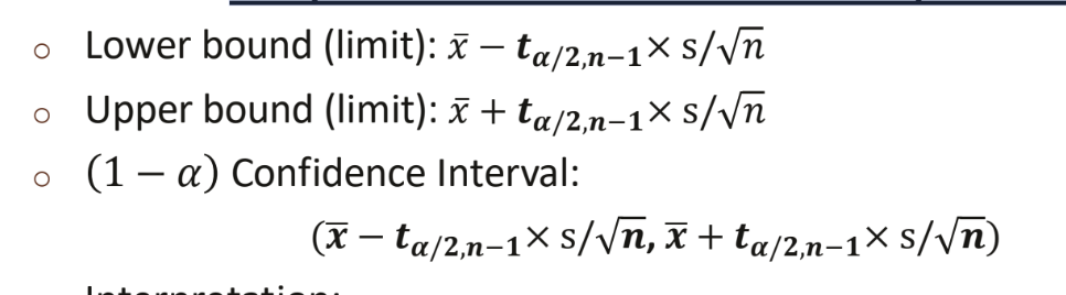
tα/2,n−1×s/ sqrt(n) is the margin of error.

• tα/2,n−1 is the cut-off (It is the actual cut-off on the t-table with the right-tail probability α/2 and the degrees of freedom n-1.)

• s/ n is the estimated standard error.

(1-α) Confidence Interval for μ: Step Three

Compute confidence interval and Interpretation

hypothesis

a declarative statement about a population, usually of the form that a certain parameter takes a particular numerical value or falls in a certain range of values.

Null hypothesis

(Hsub0) is the hypothesis we conclude to be true unless we have data that is sufficient to suggest otherwise, similar to “innocent until proven guilty”.

It often reflects existing knowledge or conventional belief.

alternative hypothesis

(Ha or H1) is the hypothesis that we conclude to be true if we have data that is sufficient to suggest the null hypothesis is not true.

Usually represents what researchers aim to demonstrate or show.

important principle of two hypotheses

One of the two hypotheses must be true, and the other must be false.

two hypothesis example: A university previously reported that at most 40% of students check social media during class. A researcher believes that with the rise of smartphones and apps, the proportion of students who check social media during class has increased.

Ha: p>0.4 vs. H0 p ≤ 0.4

btw just equal to is ok as well

two hypothesis example: A coffee shop claims that at least 80% of students feel sufficiently energized after drinking one cup of their coffee. However, you suspect the coffee is weaker than advertised and believe the proportion of students who feel energized is actually lower.

Ha: p< 0.8 vs. H0: p ≥ 0.8

two hypotheses example: About 13% of the general population is left-handed. A researcher at Lehigh University speculates that students in the Arts Departments may be more likely to be left-handed than people in the general population.

Ha: P> 0.13 vs H0: p ≤ 0.13

Hypothesis Testing

a statistical procedure that uses sample evidence to evaluate a claim about a population and determine whether there is sufficient evidence to reject the null hypothesis in favor of the alternative hypothesis:

how to go about hypothesis testing

• We begin by assuming that the null hypothesis is true.

• We examine whether the observed sample results are sufficiently unlikely under this assumption.

• If the evidence is strong enough, we reject the null hypothesis in favor of the alternative hypothesis.

• Otherwise, we fail to reject the null hypothesis due to insufficient evidence.

hypothesis testing key idea

Hypothesis testing does not prove a hypothesis is true or false. It helps us make decisions based on statistical evidence.

Right-tailed test

Ho: p ≤ po vs. Ha: p > po

left tail test

Ho: p ≤ po vs. Ha: p > po

two-sided test

Ho: p = po vs. Ha: p ≠ po

test statistic

A test statistic describes how far the point estimate falls from the parameter value given in the null hypothesis:

test statistic value

o If the test statistic is large enough in the direction specified by the alternative hypothesis, it is good evidence against the null hypothesis and in favor of the alternative hypothesis.

o We use the test statistic to compose the evidence against the null hypothesis by giving a probability , the p-value.

p value

the probability that the test statistic equals the observed value or a value even more extreme.

o It is calculated by presuming that the null hypothesis H0 is true.

p value magnitude

The smaller the p-value, the stronger the evidence the data provide against the null hypothesis.

significance level (α)

the value compared to the p-value for the conclusion. (This is also a risk tolerance of rejecting the null hypothesis when it is, in fact, true.)

The conventionally used significance level is 0.01, 0.05, or 0.1.

o We can think of this as 1 – confidence level.

Hypothesis Testing for P: Step 1

Check the assumptions

1. The variable must be categorical

2. The data should be obtained using randomization

3. The sample size is sufficiently large :

n x po ≥ 15 and n x 1 − po ≥ 15 where po is the testing value.

Hypothesis Testing for P: Step 2

state hypothesis

State Hypotheses to some value we’re interested in, po:

Hypothesis Testing for P: Step 3

Calculate Test Statistic

o The test statistic measures how different the sample proportion we have is from the null hypothesis

o We calculate the z-score by assuming that po is the population proportion (we use p = p0)

It is called the z-test statistic.

Hypothesis Testing for P: Step 4

Determine the p-value

o The p-value describes how unusual the sample data would be if Ho were true, which is what we’re assuming (p = p0)

Hypothesis Testing for P: Step 5

Make a conclusion and provide an interpretation

o Smaller p-values give stronger evidence against Ho

o α is the significance level (1- confidence level)

p-value ≤ α (significance level)

Reject H0

Under the significance level = α, there is insufficient statistical evidence to support the alternative hypothesis.

p-value> α (significance level)

Fail to reject H0 / Do not reject H0

Under the significance level = α, there is sufficient statistical evidence to support the alternative hypothesis.

Small p-value

• Your data is very unlikely to happen by random chance alone. You reject the null hypothesis and conclude your effect is statistically significant

Large p-value:

• our data could easily happen just by normal, everyday luck. You fail to reject the null hypothesis because you do not have enough proof to claim a real effect.

z test components

1. assumptions

2. - Ha: p > p_0 (right-tailed), Ha: p < p_0 (left-tailed), Ha: p ≠ p_0 (two-tailed)

3. find z score

4. P-value

   The probability of observing a test statistic as extreme as—or more extreme than—your calculated z-score, assuming H0 is true:

   • Right-tailed (>): Area to the right of z

   • Left-tailed (<): Area to the left of z

   • Two-tailed (≠ ): 2 x {area in the tail beyond |z|)

p̂ vs p0 in z test

Feature	p^​ ("p-hat")	p0​ ("p-naught" / "p-zero")
What it represents	The sample proportion (what you actually observed in your data).	The null hypothesis proportion (the benchmark or claim you are testing against).
Where it comes from	Calculated from your sample: p̂ } = x/n	Given in the problem's claim or baseline (H0: p = p0)

p vs p0

• p: The true population proportion (e.g., the actual percentage of defective items in a factory).

• p0: The specific benchmark or claimed value you are testing against (e.g., 0.05, or 5%).