RM - ALL Flashcards

Benefits of randomization

ensuring that all else is equal between treatment and control except treatment itself

How can we check our randomization?

1) checking observable characteristics of groups
2) checking whether treatment effects are similar with and without controls

Heteroskedastic errors

standard errors whose variance is correlated with the regressors (no constant conditional variance across treatment)

Homoskedastic errors

constant conditional variance across the independent variable

When is an estimate also interpreted as elasticity

when its a log-log regression

Interpretation of an elasticity

the percentage change in Y when X changes by one percent

T-value calculation

treatment estimate - (our Null hypothesis = usually 0 because we assume no effect) divided by standard error

Two elements of omitted variable bias

1) relationship between treatment and omitted variable
2) effect of omitted variable on the outcome

Calculation of OVB if you have long and short coefficient

OVB = long minus short

Interpretation of OLS regression results (if not fully randomization is ensured)

never a causal effect always just an association
= rejecting the hypothesis that there is no effect (but not saying there is one)

Two major concerns of field experiments

1) treatment dilution
2) imperfect random assignment

Treatment dilution

individuals assigned to treatment group are not treated

ITT calculation (words)

Estimate of treatment minus estimate of control

True effect for IV (word)

LATE

true effect for IV (calculation)

Intent-to-treat divided by compliance rate

Compliance rate (phi in IV) formula

Percentage of people who were assigned treatment and did treatment MINUS percentage of people who were not assigned treatment and did treatment

Ihree IV assumptions

1) Independence
2) Relevance
3) Exclusion Restriction

How to estimate a bias on the true causal effect (when we have imperfect compliance)

without treatment, how would effect look like for each group
= e.g. those who do not take the treatment might not need/want it because XY
general characteristic influences the direction (higher costs + opting in = overestimating the effect)

simple direction of bias rule (when imperfect compliance)

Baseline Trait of noncompliers and how trait affects outcome (without treatment)

Thumb rule for over/underestimating effect

Does the treatment group consist of people who are naturally better or naturally worse at the final outcome?
= tendencies of overestimating/upwards bias vs underestimating/downwards bias effect

Standard deviation

measures the variability in data
used to make differences comparable between different studies
one standard deviation difference = big jump

Mathematical expectation of a variable

the population average of this variable

statistical significance

it is highly unlikely but not impossible that difference arose purely by chance

Dealing with heteroskedasticity

using robust standard errors

Central Limit theorem

with enough data, the distribution of the t-statistic is smooth and bell-shaped (also with dummy variable)

OLS estimator (formula words)

causal + selection

beta HAT OLS estimate

beta + Cov(e,D) / Var(D)

Selection bias in OLS estimator (formula)

COV(e,D) / Var (D)

OLS estimator if we have imperfect randomization

does not reflect the causal effect of taking the treatment but is biased by a selection term

Endogeneity (words)

the covariance of the treatment and the error term is not zero = OLS problematic

Exogenous (condition + OLS)

Covariance between the treatment and the error term is 0 = OLS no problem

IV method

uses three assumptions to characterise a chain reaction leading from the instrument to outcome

Three IV assumptions

1) Relevance of the instrument
2) independence assumption
3) exclusion restriction

IV Assumption 1 - Relevance

the instrument is correlated with the treatment
COV(Z, D) is unequal 0

IV assumption 2 - Independence

The instrument is not correlated with errors

IV assumption 3 - Exclusion restriction

The instrument only affects the outcome Y through the treatment D

Testing IV assumption

1) can be directly tested via regression from data
2) & 3) cannot be directly tested, the researcher needs to argue why this holds

Instrument is strong enough when

f-statistic of first regression > 10

OLS estimator (formula)

COV(D,Y) / Var(D)

IV estimator OLS (formula)

COV (Z,Y) /COV (Z,D)

IV estimator (words)

ratio of two OLS estimators (rho and phi)

IV - Phi (formula) as OLS estimator

COV(Z,D) /Var (Z)

IV - Phi (words) & OLS estimator

Covariance of Instrument and Treatment divided by variance of Instrument

Rho (formula) - (co)variances

COV (Z,Y) / Var (Z)

IV -Rho (words)

Covariance of the Instrument and Outcome divide by Variance of Instrument

Rho also called

reduced form
intent to treat

IV - Phi also called

first stage

to get causal effect via manual IV

estimate both regressions (reduced and first stage) and divide the reduced by the first one

RHO written as Expectations (formula)

E[Y | Z = 1] - E[Y | Z = 0] 

Phi written as expectations (formula)

E [ D | Z = 1] - E[ D| Z = 0] 

RHO in terms of expectations (words)

The expected outcome of those who have the instrument MINUS the expected outcome of those without the instrument

PHI in terms of expectations (words)

The likelihood of getting the treatment when having the instrument MINUS the likelihood of getting the treatment when NOT having the instrument

Why do we need a strong first stage?

so we do not divide by zero

How does IV get rid of the selection bias?

BECAUSE of the assumption that the instrument is not correlated with the error (the thing causing selection bias)

How does the 2SLS get rid of selection bias?

using the fitted values for the treatment gets rid of the error (because fitted values are predicted values, not real ones = no error)

PHI when we have perfect compliance

is 1

IV - When Phi < 1

incomplete compliance
= the Intent to Treat is bigger than the local average treatment effect

LATE formula

gamma = rho / phi

Why are we estimating only the effect of compliers with IV?

because we only have variation in the treatment (e.g. we only observe treatment on those who otherwise would not get it)

never takers

those who would never take the treatment

always takers

those who would always take the treatment

Assumption needed to interpret IV beta as LATE

Monotonicity assumption

Monotonicity assumption

there are no defiers

Defiers

those who would only take treatment if they do not get the instrument (randomization)

Two-stage least squares

alternative way of computing ratio of rho and phi by means of a sequence of two regressions

Regression in the two-stage least squares

1) Regress the treatment on the instrument variable
2) save the predicted values from Regression 1 and regress the outcome variable on these predicted values

Advantages of 2SLS

1) allows as many control variables as you’d like
2) allows to efficiently use more than 1 instrument per exogenous covariate

Steps to 2SLS

1) test instrument
2) estimate the impact of instrument on treatment
3) Use fitted values of treatment for second-stage equation

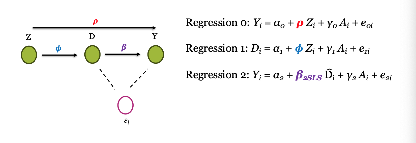
2SLS - Regression 0

Yi = a0 + rho * Zi + y0 Ai + e0i

2SLS - Regression 1 (formula)

Di = a1 + Phi * Zi + y1Ai + e1i

2SLS - Regression 2 (formula)

Y_i = a_2 + beta_2SLS* D^HAT + y_2*Ai + e_2i

Parameters in 2SLS

rho = overall effect of instrument on outcome
phi = effect of instrument on treatment
beta = true causal effect of treatment on outcome
ei = confounder that affects relationship of treatment and outcome

Def. Sharp RDD (short)

one side is treated, the other is not

Def. Fuzzy RD (short)

difference in treatment intensity to left and the right side (can use IV)

Difference- in- Difference Designs

allow you to estimate causal effects using before and after comparison in time

Causal intuition of Diff In Diff

compare the outcomes of the treatment group before and after the start of the treatment to the outcomes of the control group before and after

Basic steps of Diff in Diff (very simple)

1) Take difference treatment and control after
2) subtract difference treatment and control before
3) Hopefully this makes ceteris paribus

Basic DD regression equation

Y_dt = a + b+Tread_d + gamma Post_t + delta(Treat_d * Post_t) + e_dt

Subscript d

indicates the group (needed for Y, Treatment and error)

Subscript t

indicates the time period (needed for Y, Post and error)

Advantage of Diff in Diff

comparing changes instead of levels = eliminate fixed differences between groups that might otherwise generate omitted variable bias

Manual calculation of DD estimate (formula)

(Y_1_t - Y_0_t) - (Y_1_t-1 - Y_0_t-1)

Manual calculation of DD estimate (words)

subtracting pre-treatment differences between two units from the post treatment differences

DD counterfactual

from strong assumption of common trends

Time effects

capture temporal changes in the outcome variable that are common to all units of observation

Group effects

difference between treatment and control group before the treatment

Interpretation alpha in Diff-in-Diff

constant
outcome for the control group in the pre-reform period

Interpretation beta (Group dummy)

difference between treatment and control before treatment

Interpretation gamma (Time dummy)

common difference in outcome for treatment and control group in post-reform period (seen in control group slope)

Interpretation delta ( Treatment effect/Interaction term dummy)

difference in outcome for treatment and control group in post-reform period MINUS the difference in outcome of treatment and control group in the pre-reform period

Extended DD Regression equation (only more time dummies)

Y_dt = alpha + beta Tread_d + SUM_s(gamma_s POST_s) + delta(Treat_d + Post_t) + e_dt

Extended DD Regression (year and treatment dummies)

Y_dt = alpha +beta Treat_d + SUM_s(gamma_s Post_s) + SUM_u(delta_u (Treat_d * Post_u) + e_dt

Why include multiple dummies in Diff-in-Diff

to capture individual year effects
and to capture build up of treatment

How to account for different trends of treatment and control group in Diff in Diff

adding differential trends (e.g. demographic characteristics that change over time)

Notation differential trends

n_treat( Treat_d * t)
n_control(Control_d * t)

Adding control variable notation

pi * Xi (vector of control variables)

Key assumptions of DD

1) common time effects
2) exogeneity of the reform
3) No anticipation of the reform

Common time effects assumption

In absence of the reform both groups would have evolved parallel

Exogeneity of the reform

reform not related to different development of treatment and control group

No anticipation of the reform

Treatment group did not respond before the reform