ECON Exam 2 (Ch. 7-10)

Covers Ch. 7 - "The Aggregate Demand and Aggregate Supply Model" , Ch. 8 - "Introduction to the Classical Model" , Ch. 9 - "Introduction to the Keynesian Model", and Ch. 10 - "Government in the Macroeconomy: Fiscal Policy"

Aggregate Demand (AD)

C+I+G+(X-M) = C+I+G+NX

Shows the relationship between the quantity demanded of all goods and services produced in the domestic economy and the price level (ceteris paribus).

= Real GDP (in a long-run equilibrium) (actual GDP equals aggregate demand only when the economy reaches a long-run equilibrium)

Positive changes in Aggregate Demand (AD)

indicated by shifts to the right

1) Decrease in interest rates

2) Increase in wealth

3) Increase in confidence

4) Decrease in taxes

5) Increase in government transfer payments

6) Increase in government spending

7) Increase in foreign real national income

8) Depreciation of the dollar

Negative changes in Aggregate Demand (AD)

Leftward shift in the graph

1) Increase in interest rates

2) Decrease in wealth

3) Decrease in confidence

4) Increase in taxes

5) Decrease in government transfer payments

6) Decrease in government spending

7) Decrease in foreign real national income

8) Appreciation of the dollar

An increase in AD (rightward shift) leads to:

An increase in the price level and an increase in output.

A decrease in AD (left shift) leads to:

A decrease in the price level and an decrease in output.

Short-run Aggregate Supply (SRAS)

shows the relationship between the quantity supplied of real GDP and the price level (ceteris paribus).

Primary factors that cause SRAS shifts in change

1) Change in price of an input (Wage rates or energy prices), which change costs of production

2) Supply shocks

Factors that cause positive SRAS (rightward shift) change:

1) Lower input prices (wage rates or energy prices), leads to lower costs of production

2) Positive (beneficial) supply shock

An increase in Short Run Aggregate Supply (SRAS) leads to

(shifting rightwards)

A decrease in the price level and an increase in output.

A decrease in SRAS (shifting left) leads to

An increase in the price level and a decrease in output.

Positive (Beneficial) Supply Shock

A sudden, unexpected event that increases the availability of goods or services or lowers production costs across an economy. (leads to an increase in SRAS)

Negative (Adverse) Supply Shock

A sudden, unexpected event that reduces the availability of goods or services or sharply increases production costs across an economy. (leads to a decrease in SRAS)

Potential Real GDP (natural real GDP [Q_N])

It is the "Sweet Spot": Potential GDP is the maximum amount of goods and services an economy can produce sustainably over time when using all its available resources (labor, capital, technology) at normal (noncyclical rate) employment.

Is the amount of output produced when the economy is operating at the noncyclical (natural) rate of unemployment.

Potential Real GDP on Graph (LRAS)

Represented by a vertical line at the maximum sustainable amount of output.

GDP Gap

When actual real GDP is not equal to potential (natural) real GDP.

This indicates whether the economy is likely to expand or contract in the short run.

3 possible relationships between actual real GDP (Q_E) and potential (or natural) GDP (Q_N) at any point in time:

• Q_E = Q_N (Full-Employment Equilibrium)

• Q_E > Q_N (Inflationary Gap)

• Q_E < Q_N (Recessionary Gap)

Full-employment equilibrium

No GDP gap, the economy is at full employment, actual real GDP is equal to potential (or natural) real GDP (Q_E = Q_N), and unemployment rate is equal to the noncyclical (natural) rate (U = U_N).

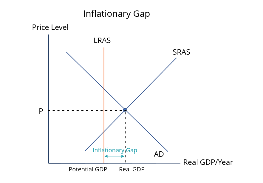
Inflationary Gap

The economy can produce a level of output higher than the potential (natural) real GDP (Q_E < Q_N) by ‘overemploying’ resources and the unemployment rate is less than the noncyclical (natural) rate (U > U_N).

Recessionary Gap

The economy operates below full potential.

Actual real GDP is below potential (natural) real GDP (Q_E < Q_N), the actual unemployment rate is higher than the noncyclical (natural) rate (U > U_N).

Economic Growth in AD and AS

LRAS curve shifts to the right and increase in AD (right shift) without inflation.

Adam Smith (Classical Model)

Wrote Wealth of Nations in 1776, where Smith argues:

• Favor of free trade

• Free markets

• A small role for government in market interactions

Invisible Hand

When individuals pursue their own self-interest, they put their resources to the highest-valued use, which unintentionally promotes the public interest.

Assumptions of the Classical Model

Three basic assumptions for a capitalist economy:

• Flexible prices, wages, and interest rates

• Saving equates with investment

• Say’s Law is true

Classical Model (Summary of Assumptions)

• Flexible prices (Goods and services market) ensure that output markets clear.

• Flexible wages (Labor market) cause the labor market to adjust to eliminate labor shortages and labor surpluses.

• Saving and investment are equated because of flexible interest rates (loanable funds market).

• Law’s Law explains “supply creates its own demand”

The Classical Model states:

A market economy self-corrects when it deviates from its long-run equilibrium at full employment.

Keynesian View

Argues that a market economy can settle at an equilibrium below full employment.

John Maynard Keynes (Keynesian Revolution)

Wrote The General Theory of Employment, Interest, and Money (1986) where Keynes argued:

• When national economies suffer downturns, governments should borrow and spend money to boost economic activity.

• Once the intervention produces the desired outcome of economic growth, government should no longer be actively involved.

Price level (Keynesian)

The Keynesian Model assumes that the price level is “sticky” and not likely to rise or fall in the short run.

Disposable Income

The income available to households to spend or save after paying taxes (T).

Keynesian Consumption Function

Consumption is a function of disposable income.

• Consumption spending (C) depends on disposable income (Y_D).

Two components to consumption

1) Autonomous consumption (C₀)

2) Induced consumption (MPC(Y_D) )

Autonomous Consumption (C₀)

The minimum spending a household must make even if its disposable income drops to zero.

Induced consumption, MPC(Y_D)

The additional consumption spending that occurs as disposable income increases.

Keynes’ “Propensity to consume” assumptions:

• Argued that people have a “propensity to consume”, which includes making provisions for future consumption.

• Believes that propensity to consume is stable in the short run

• Implies consumer spending that occurs as a result of a change in disposable income can be predicted from the marginal propensity to consume (MPC).

Marginal Propensity to Consume (MPC)

The proportion of an additional increase in income that a consumer spends on goods and services rather than saving

Marginal Propensity to Save (MPS)

The amount of disposable income that goes to saving.

Break-even disposable income

Determined at what level of income all disposable income is spent and saving is equal to 0.

• if all income is spent, C = Y_D, so S must be 0.

The Autonomous Spending Multiplier (Spending Multiplier)

Tells the increase in equilibrium income that occurs due to a $1 increase in autonomous spending.

The Core Concept: Money Keeps Moving

Imagine you spend $100 at a local coffee shop. That $100 isn't the end of the story—it becomes income for the coffee shop owner and baristas.

1. Round 1: You spend $100 at the coffee shop.

2. Round 2: The coffee shop owner takes that $100 and uses $80 of it to pay a local baker for pastries (saving $20).

3. Round 3: The baker takes that $80 and spends $64 at the hardware store (saving $16).

4. Round 4: The hardware store owner spends $51.20...

Notice how your original $100 injected into the economy generated $100 + $80 + $64 + $51.20 = $295.20 (and counting) in total spending across the economy.

Fiscal Policy

The use of the government’s budget to influence macroeconomic outcomes to help achieve the goals of full employment, price stability, and economic growth.

Discretionary Fiscal Policy

When Congress passes a new legislation that changes government spending.

Automatic (Nondiscretionary) Fiscal Policy

Ongoing government programs that trigger automatic changes in government.

Expansionary fiscal policy

Increases in government spending and decreases in taxes, when the economy is in a slump and a recession may occur.

Contractionary fiscal policy

Decreases in government spending and increases in taxes, when the economy is overheating and an inflation may occur.

Balanced Budget

If government spending is equal to tax revenues. (G = T)

Budget Deficit

If government spending is greater than tax revenues. (G > T)

Budget Surplus

If government spending is less than tax revenues. (G < T)

Fiscal Policy assumptions:

• A fixed price level

• A constant and known MPC

• Consumption depends on disposable income

• Investment spending and government spending are autonomous

• Tax changes are lump sum

Lump sum tax

A fixed tax amount regardless of an individual’s income or consumption.

Crowding Out

Occurs when increased public sector activities reduces private sector activities.

Proportional Income Tax

Constant tax rate for all levels of income.

Progressive Income Tax

Tax rate increases as income increases.

Regressive Income Tax

Tax rate decreases as income increases.