Psy 201 lecture 2

Sampling from a population

normal distribution or Gaussian distribution

particular probability distribution that

displays this “bell curve” shape. It is symmetric, and about 66.67% of data is within ±1 SDs.

Importantly, this shape manifests in nature

uniform distribution

where all scores occur in relative equal frequencies

multimodal or shapeless distribution

has no discernable shape

Kurtosis

where the distribution is normal-ish, but the spread is either more or less than

2/3rds of scores are within ±1 SD from the mean

Kurtosis - leptokurtic

more than 2/3 within +-1 SD

Kurtosis - platykurtic

scores are spread out, less then 2/3 within +- 1 SD

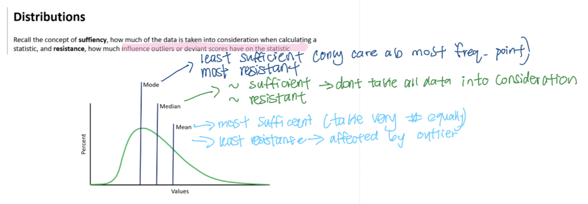
sufficiency and resistance of mean mode and median

central tendency formulas for both pop mean and sample mean

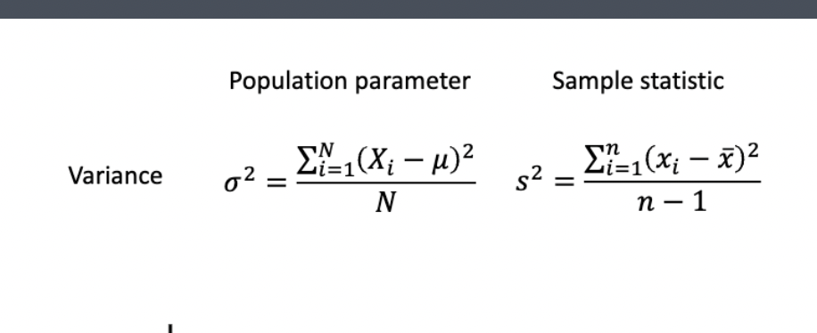
why we divide sample statistics by n-1 —> theoretical reason

in order to make sample variance unbiased one score must be accounted for. If n scores are sampled, n – 1 can be any score, but the nth score must be controlled for to ensure sample variance is not an underestimation. By dividing over n – 1, we are removing the influence of one of the scores

why we divide sample statistics by n-1 —> algebraic reason

the lower the n, the more extreme the underestimation. This is proportional to n, specifically 1/n. Thus, an n of 10 will have a 10% bias, which corresponds to 1 out of 1. An n of 100 likely has a 1% bias, which still corresponds to 1 out of 10

sampling distributions: central limit theorem three rules

1. Regardless of sample size, the average of the sample means are very close to the population mean

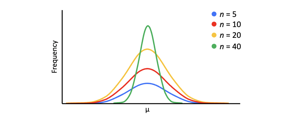
2. Larger sample sizes have less variability in their sample statistic than do smaller sample sizes

3. The accuracy of sample standard deviation improves as sample size increases

central limit theorem

states that as n increases, a sample of sample means (i.e., a sampling distribution) will approach a normally-shaped distribution no matter what the original population’s shape is

sampling distribution

At 10,000 samples of each sample size, you can really see how samples with larger ns have means that are less spread out. The larger your n, the closer the sample mean will likely be to the population mean and the more consistently this will occur.

standard error of the mean

The standard error of the mean is the shortcut to calculating standard deviation of a sampling distribution at a given sample size, and tells you where the population mean likely lies in relation to the sample mean

• tells you how accurate your sample mean is to the population mean. It is a measure of statistical accuracy

z score

standardized score which describes the distance in standardized

units between a value (e.g., a mean or single score) and the distribution (i.e., population) mean. The shaded area under the curve is the probability of being above that score (i.e., smaller portion of the distribution)

grand mean

average of all scores across conditions, is just the average of the condition means. This only works if the ns are equal. If the ns are unequal, you have to reweigh the means. Groups with larger ns have more weight. This is the same for reweighing variance