biostats - Chapter 10

Normal distribution

a continuous, probability distribution describing a bell shaped curve

• good approximation to the frequency distributions of many biological variables

• two parameters mean standard deviation

Properties:

• Continuous distribution, so probability is measured as area under the curve

• It is symmetrical around its mean (bell-shaped)

• Single mode

• Probability density is highest exactly at the mean

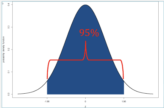
Normal distribution symmetry

For a variable with a normal distribution, about about two thirds of samples are within one standard deviation, and about 95% of samples are within two standard deviations

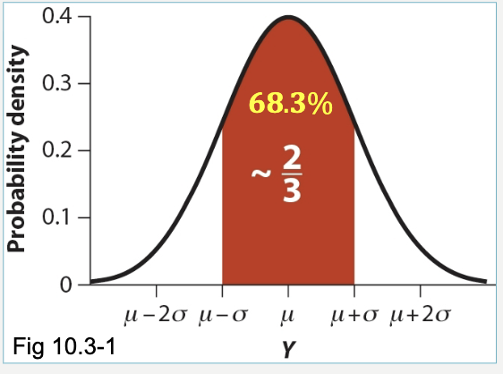
• 2/3 of the data are in one Standard deviation

• mean is at standard deviation = 0

• 95% is within 3 standard deviations

Standard normal distribution

The standard normal distribution is a normal distribution with a mean of zero and a standard deviation of one

• Indicated by symbol Z

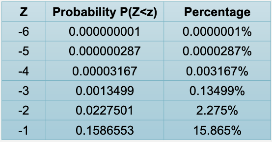
Probability that a random draw from the standard normal distribution is above a given Z

Since distribution is symmetrical around mean, the probabilities of negative Z values are the same as the positive Z values

Why standard normal distribution

• There are an infinite number of normal distributions, but they are all similar in shape (i.e., bell curve)

• Able to transform for probability calculation under a standard normal distribution

• A standard normal deviate, or Z, tells us how many standard deviations a particular value is from the mean

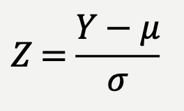
Positive means above mean; negative means below mean

A really low or really high Z score suggest implausible data

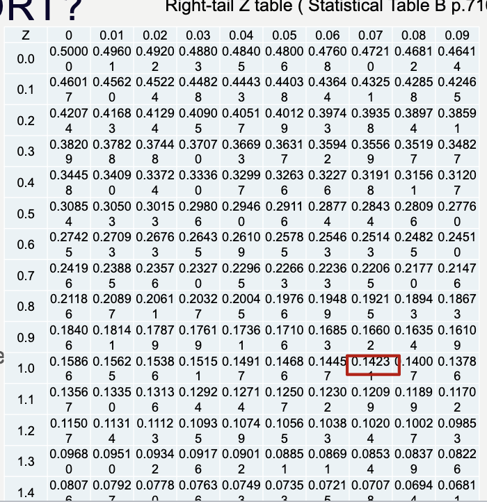
To find the probability of a sample mean, we first convert the value to a Z- score and then look up this value in the Z-table. The table shows the probability of observing a value greater than this Z-score under the normal distribution

Example Problem

A sample of 50 students took a statistics quiz.

Mean score: 70; Standard deviation: 8

1) Calculate the z-score for a student who scored 82.

2) Is the score above or below the mean?

3) How many standard deviations away is it?

score is above the mean

1.5 Z away

Example Problem

In a study of adult BMI (kg/m2).

Mean BMI: 26 kg/m2;

Standard deviation: 4 kg/m2

(Z-score is good here because it helps get rid of and identify implausible values)

1) Calculate the z-score for someone with BMI = 34 kg/m2.

2) Is the score above or below the mean?

3) How many standard deviations away is it?

Score is above mean

Example Problem

In a population study of adult females, the average height is:

Mean height: 163 cm;

Standard deviation: 6 cm

1) Calculate the z-score for someone with height = 100 cm.

2) Is the score above or below the mean?

3) How many standard deviations away is it?

Z = - 6.33

This is below the mean

Data may be implausible

Example Problem NASA

NASA has height restrictions for astronaut pilots

157.5 cm (62 inches) ≤ height ≤ 190.5 cm (75 inches)

1) What fraction of the US population is excluded?

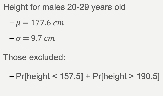
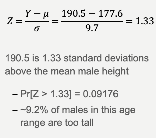
Males too tall:

Males too short:

Excluded males: (either too short or too tall) ADDITION RULE

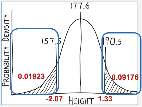
Approximately 11.1% of men would be excluded from NASA's height requirements because they are either shorter than 157.5 cm or taller than 190.5 cm

Normal distribution of sample means

• Normal distribution can be used to describe the sampling distribution of many estimates, including the mean

• The sampling distribution is the probability of all values for an estimate that we might obtain when we sample a population (from chapter 4)

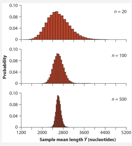
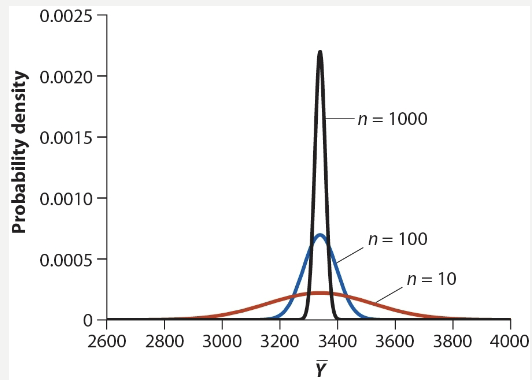
If a variable Y has a normal distribution in the population, then the distribution of the sample means Y is also normal.

Increasing the sample size reduces the sample error and increases the precision of the distribution of sample means

Example Problem:

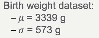
Suppose random sample of 80 babies produces a mean of 3370

1) What is the probability getting mean of 3370 or greater?

0.48 standard deviations away

Z = 0.48

To find the probability of a sample mean greater than 3370, we first convert the value to a Z- score (0.48) and then look up this value in the Z-table. The table shows the probability of observing a value greater than this Z-score under the normal distribution

Using table: Approximately 31.6% of random samples of 80 babies would have a mean birth weight of 3370 g or greater.

Central Limit Theorem

• According to the central limit theorem, the sum or mean of a large number of measurements randomly sampled from a non-normal distribution is approximately normal

• Many statistical tests that assumes the distribution of means is normal

• So central limit theorem allows use of these tests even if the distribution of the sampled population parameter is not normal

• How many samples needed depends on shape of the distribution of observations

  

The Central Limit Theorem allows us to approximate a binomial distribution with a normal distribution when the sample size is large.

The normal approximation works well when:

• These conditions ensure the binomial distribution is not too skewed.

Interpretation:

In hypothesis testing, we compare the p-value with the significance level (α=0.05)

If p < α → Reject H0

I f p ≥ α → Fail to reject H0

Example Problem

Researchers studied whether brown recluse spiders prefer dead crickets

Sample:

• n = 41

• x successes (dead crickets) = 31

Null hypothesis: H0: p = 0.5 (no preference)

Alternative hypothesis: HA: p≠0.5 (is different)

(two-sided test)

P (X ≥ 31)

1) Find the mean and standard deviation

2) Continuity correction

3) Convert to Z-score

4) Find the probability and interpret

If :

2) Then the approximating normal distribution has:

The binomial distribution is discrete, while the normal distribution is continuous.

To improve the approximation, we apply a continuity correction of ± 0.5.

P (X ≥ 31)

2) Continuity Correction

= 31 - 0.5 = 30.5

3) We convert the value to a z-score using:

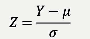
Where:

• Y = observed value (corrected x) = 30.5

• μ = 20.5

• σ = 3.20156

4) Then we use the standard normal table to find probabilities.

Using the Z-table:

P(Z > 3.12) ≈ 0.0009

Because this is a two-sided test (we multiply by 2):

P = 2× 0.0009 = 2 x 0.0009 = 0.0018

Interpretation:

Since the p-value (0.0018) is smaller than the significance level (α = 0.05), we reject the null hypothesis.

There is statistical evidence that brown recluse spiders prefer one type of prey.

Review: Hypothesis testing

Like estimation, uses sample data to make inferences about the population from which the sample was taken.

Unlike estimation, however, which puts bounds on the value of population parameter, hypothesis testing asks only whether the parameter differs from a specific “null” expectation.

• Estimation asks, “How large is the effect?”

• Hypothesis testing asks, “Is there any effect at all?”

In hypothesis testing, when do we use a two-sided test versus a one-sided test?"

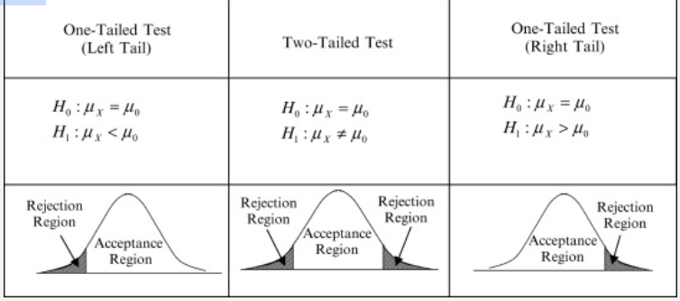
• One over the other, or under the other means one-sided

• Different means 2 sided

In hypothesis testing we compare the p-value with the significance level (α=0.05 = 5%)

• If p < α → Reject H0

• If p ≥ α → Fail to reject H0

Review: Proportions

Proportion of observations in a given category

• Ranges from 0 to 1

Confidence interval of proportion

• Different methods of calculation exist

• Confidence intervals provide an alternative to hypothesis testing

  • Agresti-Coull method

95% confidence interval

• if Interval does not include the null proportion of 0.5, and in fact is well abovethe null then data are inconsistent with the null

Review: Goodness-of-fit test

Goodness-of-fit test: method of comparing an observed frequency distribution with the frequency distribution expected under a probability model.

• Binomial test is an example of a goodness-of-fit test.

• What is the limitation of the binomial test?

- Must fit into two mutually exclusive outcomes (success and failure)

The X2 goodness-of-fit test compares frequency data to a probability model stated by the null

• More general than the binomial test because it can handle more than two categories

• Calculations also easier

The X2 test statistic measures the discrepancy between observed frequencies from the data and expected frequencies from the null hypothesis

Degrees of freedom and critical value (α = 0.05) are compared to the calculated X²

• if calculated value is smaller, you fail to reject H0

• if same size, you reject H0

Review: 2X2 contingency tables

Three different ways to analyze these data

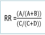
1. Relative risk

• is the probability of an undesired outcome in the treatment/exposed group divided by the probability of the same outcome in a control/not exposed group

• Relative Risk is the "gold standard" for:

  • Longitudinal Studies: You start with a group of healthy people, divide them by exposure (e.g., smokers vs. non-smokers), and follow them forward in time.

  • Randomized Controlled Trials (RCTs): You compare the risk of an outcome in the treatment group versus the control group.

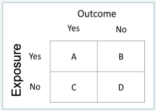
2. Odds ratio

• The odds of success are the probability of success divided by the probability of failure

• 
  

  

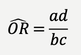
  • If O = 1 then there the odds of successes and failures are equal, thus no contingency between variables

• Use the Odds Ratio when:

  • Case–control studies

  • Cross-sectional (rare outcome < ~10%)

  • Logistic regression models (binary, ordinal, or multinomial)

  

3. X² contingency test

• Testing the association between two categorical variables

  • multiple categories