Elasticity

Price elasticity of demand

Price elasticity of demand (尸ED) is a measure

of the responsiveness of the quantity of a

good demanded to changes in its price. PED

is calculated along a given demand curve.

In general' if quantity demanded is highly

responsive to a change in price, demand is

referred to as being price elastic; if quantity

demanded is not very responsive, demand is

price inelastic.

Formula for PED

Sign of PED

PED is used as a positive number even though values may be negative. - Absolute value is considered.

Use of percentages

1. We need a measure of responsiveness that is

   independent of units. 

2. It is meaningless to think of changes in prices or

   quantities in absolute terms 

Range of values for PED

Demand is price inelastic when PED<1 (but greater

than zero). The percentage change in quantity

demanded is smaller than the percentage change in

price, so the value of PED is less than one; quantity

demanded is relatively unresponsive to changes in

price, and demand is price inelastic. 

Demand is price elastic when PED>1 (but less

than infinity). The percentage change in quantity

demanded is larger than the percentage change

in price, so the value of PED is greater than one;

quantity demanded is relatively responsive to price

changes, and demand is price elastic. 

Unitary elasticity

Demand is unit elastic when PED = X. The percentage

change in quantity demanded is equal to the

percentage change in price, so PED is equal to one;

demand is then unit elastic., there is unitary PED.

Perfectly inelastic

Demand is perfectly inelastic when PED - 0. The

percentage change in quantity demanded is zero;

there is no change in quantity demanded, which

remains constant at Q\ no matter what happens to

price; PED is then equal to zero and demand

is perfectly inelastic

Perfectly elastic

Demand is perfectly elastic when PED = infinity.

When a change in price results in an infinitely

large response in quantity demanded, demand

is perfectly elastic

Steepness of curve and PED

We often use the relative steepness of demand

curves to be an indication of PED, so that

comparing two demand curves, the one that is

flatter is said to be more elastic while the one

that is steeper is said to be more inelastic. 

Varying PED on a demand curve

On any downward-sloping, straight-line

demand curve, demand is price-elastic at high

prices and low quantities, and price-inelastic at

low price and large quantities. At the midpoint

of the demand curve, there is unit elastic

demand.

Therefore, the terms 'elastic' and 'inelastic'

should not be used to refer to an entire

demand curve (with the exception of the

three special cases where PED is constant),

but only to a portion of the demand curve

corresponding to a particular price or

price range.

Determinants of PED

1. Number and closeness of substitutes

2. Necessities vs luxuries

3. Length of time

4. Proportion of income spent on a good

Total revenue

Total revenue (TR) is the amount of money received by

firms when they sell a good (or service), and is equal to

the price (P) of the good times the quantity (Q) of the

good sold. Therefore, TR - P^Q.

PED and total revenue

When demand is elastic, an increase in price

causes a fall in total revenue, while a decrease in

price causes a rise in total revenue.

When demand is inelastic, an increase in price

causes an increase in total revenue, while a

decrease in price causes a fall in total revenue.

When demand is unit elastic, a change in price

does not cause any change in total revenue.

PED and indirect taxes

The lower the price elasticity of demand for the

taxed good, the greater the government tax

revenues.

PED in relation to primary commodities

Many primary commodities have a relatively

low PED (price inelastic demand) because

they are necessities and have no substitutes

(for example, food and oil). The PED of

manufactured products is relatively high

(price elastic demand) because they usually

have substitutes.

Income elasticity of demand

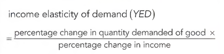
Income elasticity of demand (YED) is a measure

of the responsiveness of demand to changes

in income, and involves demand curve shifts. It

provides information on the direction of change

of demand given a change in income (increase

or decrease) and the size of the change (size of

demand curve shifts).

Income elasticity of demand - formula

Income elasticity of demand interpretations

YED>0. A positive income elasticity of

demand indicates that the good in question

is normal; demand for the good and income

change in the same direction (both increase

or both decrease).

YED<Q. A negative income elasticity of

demand indicates that the good is inferior:

demand for the good and income move in

opposite directions (as one increases the

other decreases). Examples include bus

rides, used clothes and used cars; in these

cases, as income increases, the demand

for these goods fall as consumers switch to

consumption of normal goods

Income elasticity of demand - necessities vs luxuries

YED < 1: Necessities. If a good has a YED

that is positive but less than one, it has

income inelastic demand: a percentage

increase in income produces a smaller

percentage increase in quantity demanded.

Necessities are income inelastic goods.

YED > 1: Luxuries and services. If a good

has a YED that is greater than one, it has

income elastic demand: a percentage

increase in income produces a larger

percentage increase in quantity demanded.

Luxuries and services are income elastic.

Engel curve

The Engel curve shows a continuum: at very low

incomes a good may be a luxury; as income

increases it becomes a necessity and finally at

high income levels it becomes inferior.

With income on the vertical axis and quantity on

the horizontal axis of an Engel curve diagram,

we can see the following:

YED>0 in the upward sloping part of the

curve showing quantity and income both

increasing, which indicates the good is normal

YED<0 in the downward sloping part

showing quantity decreasing as income

increases, which indicates the good is inferior.

YED and producers:

• Income Elastic Goods (YED>1): Demand grows faster than the rate of income growth (e.g., restaurants, travel, health care), leading to rapid industry expansion. However, these industries suffer the largest sales drops during a recession.

• Income Inelastic Goods (YED<1): Demand grows slower than income growth (e.g., food, clothing, furniture), leading to slower industry expansion. During a recession, these products are more stable and avoid major declines in sales.

• Inferior Goods (YED < 0): Demand actually increases during a recession when incomes fall.

YED and the sectoral structure of the economy

• Primary Sector (Agriculture, forestry, fishing, mining): Has a low YED (YED<1) because demand for food grows slower than income, and raw materials (like cotton and rubber) are often replaced by synthetic substitutes. As a result, its share of the total economy shrinks over time.

• Manufacturing Sector (Cars, TVs, computers): Has a high YED (YED>1), meaning demand grows faster than income, causing the sector's share of the economy to expand.

• Services Sector (Travel, banking, health care, education): Has the highest YED, causing demand to grow the fastest. With continued economic growth, services eventually expand at the expense of both agriculture and manufacturing.

PES

Price elasticity of supply (尸ES) is a measure

of the responsiveness of the quantity of a

good supplied to changes in its price. PES

is calculated along a given supply curve.

In general, if there is a relatively large

responsiveness of quantity supplied, supply is

referred to as being elastic; if there is a relatively

small responsiveness, supply is inelastic.

PES Formula

Supply = price inelastic

 Supply is price inelastic when PES<1. The

percentage change in quantity supplied is smaller

than the percentage change in price, so the value of

PES is less than one; quantity supplied is relatively

unresponsive to changes in price, and supply is

price inelastic or inelastic.

Supply = price elastic

Supply is price elastic when PES>1. The percentage

change in quantity supplied is larger than the

percentage change in price, so the value of the

PES is greater than one; quantity supplied is

relatively responsive to price changes, and supply

is price elastic or elastic. 

Supply = unit elastic

Supply is unit elastic when PES = 1. The percentage

change in quantity supplied is equal to the

percentage change in price, so PES is equal to

one; supply is unit elastic; there is unitary PES.

Supply is perfectly inelastic

Supply is perfectly inelastic when PES = 0. The

percentage change in quantity supplied is zero;

there is no change in quantity supplied no matter

what happens to price; PES is equal to zero and

supply is said to be perfectly inelastic. 

Supply is perfectly elastic

Supply is perfectly elastic when PES = infinity. The

percentage change in quantity supplied is infinite;

any change in price leads to an infinitely large

response in quantity supplied; supply in this

case is called perfectly elastic

Determinants of PES

1. Length of time

2. Mobility of FOPs

3. Spare (unused) capacity of firms

4. Ability to store stocks

5. Rate at which costs increasing

PES in relation to primary commodities and manufactured products

Reasons for Low PES in Primary Commodities:

• Agriculture: Farmers need at least one full planting season to adjust output. Furthermore, suitable farmland is limited or shrinking due to soil depletion, meaning higher output requires slow, costly technological advances (like better seeds and irrigation systems) amidst growing water shortages.

• Oil, Gas, and Minerals: Extracting natural resources requires massive upfront investment and setup time, so firms wait for severe shortages before committing to increasing production.

Consequences of Low PES:

• Because supply cannot easily adjust in the short term, shifts in demand cause sharp price fluctuations.

• Combined with price inelastic demand (PED), this leads to highly unstable revenues and incomes for farmers and primary producers compared to manufacturers.

Short term and long term PES

• Short Term (Low PES): Producers cannot quickly adjust their output in response to price changes due to fixed planting seasons and resource constraints, resulting in inelastic supply.

• Long Term (Higher PES): Given more time, producers can make necessary adjustments (such as investing in new technology, acquiring land, or shifting resources), making the quantity supplied much more responsive to price changes.