Business Analytics MIDTERM

you got this

unsupervised learning

data is mined to uncover previously unknown patterns w/o a clear outcome in mind

• No dependent variable to predict (no regression)

• Exploratory in nature (only provide initial direction)

• “good results” are subjective

association rule mining

find out which items tend to occur/appear together

• aka affinity analysis or market basket analysis

  • used to find out which products tend to be purchased together

  • main application = recommendations

U

universal set of items in a given domain

• ex. all the items in a grocery store

X

an item-set; any subset of U

• ex. {coffee, bagel}

• CANNOT contain duplicate items

transaction

instance of an item-set

• multiple of these comprise a dataset

• ex. all combos of products bought by different customers (each row of the dataset)

association rule

describes the relationship between item-sets; DIRECTIONAL

• X → Y: “if X, then Y”

  • X = antecedent (or body), Y = consequent (or head)

• “we recommend Y to the customer that bought X”

• X and Y can contain any number of items, but they must NOT be overlapping item-sets

support count (σ)

raw count of transactions in your dataset that contains the item-sets

support percentage (S)

fraction of transactions that contain an item-set or a pair of item-sets; NOT DIRECTIONAL

• can be for an individual item-set [ex. S(X)] or an association rule [S(X→Y)]

• highest (S) = occurs most frequently in the data set

confidence

considering X→Y, measures how often items in Y appear within transactions that contain X; DIRECTIONAL

• “given that a customer buys X, there is a (conf)% probability that they will also buy Y”

lift

how much more likely 2 item-sets co-occur than pure chance; NOT DIRECTIONAL

• >1: those who buy X are more likely to buy Y than other customers

• =1: those who buy X are as likely to buy Y as any other customers

• <1: those who buy X are less likely to buy Y than other customers

"Does this rule show an actual association, or is the confidence just pure chance?"

real association or coincidence

high confidence is not enough the prove real association → must use lift

• High Confidence can reflect general product popularity rather than a real relationship, creating high confidence even with zero true dependency

  • ex. high-frequency items like 90% bread and 95% milk will naturally co-occur by pure chance

• Use Lift to measure whether items occur together more often than expected by random chance

apriori alogrithm

if item-set X is not frequent (doesn’t satisfy the minimum threshold), then any larger item sets containing X cannot be frequent

• how we find “good” candidates with so many possible item-set combos

frequent item-set

Item sets for which support >= minsupp; combos that occur with higher frequency in the dataset

• minsupp decided based on domain knowledge or business goals

steps for apriori algorithm

1. compute support for all the 1 item-sets and keep only the frequent ones

2. form 2 item-sets using only frequent item-sets from (1) and keep only the frequent ones

3. form 3 item-sets, using only frequent item-sets from (2) and keep only the frequent ones. Keep forming N-item-sets and keeping only the frequent ones.

4. find all the items that satisfy support >= minsupp

5. generate all possible association rules (cannot have overlapping items) and calculate their confidence. Final set of rules are ones where confidnece >=minconfidence

clustering

organizing data points/observations into most natural groups called clusters

• form of unsupervised learning = observations are not pre-defined, they are discovered from the data

  • no clear outcome in mind

• evaluated and interpreted after clusters are discovered by the algorithm

desired properties of a cluster

• high intra-similarity: points in a cluster should be similar

• low inter-similarity: points in different clusters should be different

applications of clustering

1. discover natural groups and patterns in the data (ex. similarly behaving customers)

2. facilitate the analysis of very large datasets

distance measures

to measure similarity between individual data points

- numerical data - euclidian and manhattan

- binary data - matching and jaccard

the higher the distance, the more different the 2 points

euclidian distance

straight line distance b/w 2 points

• for numerical data

manhattan distance

restricts distance measurement to horizontal and vertical paths

• for numerical data

matching distance

# of mismatches / TOT # of attributes (k)

• used for symmetric binary data (N00 and N11 are equally important)

• for binary data

jaccard distances

# of mismatches / TOT # of attributes (k) —EXCLUDING matches with N00

• used for asymmetric binary data (N00 is not as important as N11)

  • mutual presences are more important than mutual absences

data normalization

eliminates specific units of measurement and transforms the attributes to a common scale. Use for:

• mixed data: when datasets have different types of attributes (numerical and binary columns)

• non-comparable data: attributes that have values in different ranges (ex. age and income)

can apply numerical distance measures after data is normalized

data normalization methods to scale attributes

• min max normalization: rescale attributes to have values between 0-1 using the min and max

  • A point with value X will be normalized to: NewValue = (X – min) / (max – min)

• standardization: transform each attribute to have mean=0 and sd=1

  • NewValue = (X – Sample mean) / (Sample standard deviation)

linkage methods

to measure similarity between clusters

• single, complete, average, centroid, and ward

single linkage

minimum pairwise distance b/w points from 2 different clusters

• very sensitive to outliers

• good for non-convex shapes

  • can produce long, straggly clusters

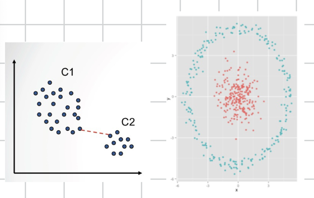
convex shape

straight line segment connecting any 2 points inside the cluster lies entirely within the cluster

complete linkage

max pairwise distance b/w points from 2 different clusters

• sensitive to outliers

• tends to break large clusters to create clusters with similar diameter

average linkage and centroid distance

average pairwise distance b/w points from 2 different clusters VS distance b/w 2 clusters’ centroids (average of all points)

• produce similar results

• create spherical shaped clusters

• less sensitive to outliers than single or complete

Ward’s method

minimize within-cluster variance b/w centroid and cluster points

• robust to outliers

• create denser clusters with spherical shapes

• best at finding underlying structure

• most computationally complex

hierarchical clustering

forming larger clusters from smaller ones; # of clusters NOT pre-specified

- aka agglomerative or bottom-up

- each data point starts as its own cluster, and points/clusters merge based on the distance measure and linkage method specified → repeats until there is only one cluster left

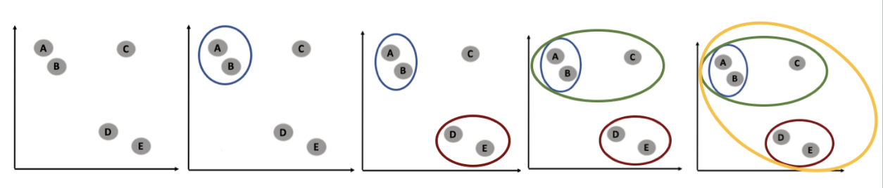
distance matrix

contains all pairwise distances b/w data points in your dataset

• fed into an algoritm and used to decide which points to hierarchically cluster

hierarchical clustering pros and cons

pros

• flexible, data-driven, no need to pre-specify the # of clusters

• produces a solution for different #s of clusters

• good at identifying “small” clusters

cons

• computationally demanding → not scalable

• can be sensitive to outliers depending on linkage method used

dendogram

diagram that shows the cluster’s hierarchy

• height of horizontal bar = merge order (higher up = formed later)

  • break clusters up from the one that was formed last

partitioned based clustering

produce specified # of clusters with the lowest within-cluster variance, where k is chosen beforehand

• most common approach = k-means clustering

• usually implemented using Euclidian distance

• keep reassigning points to the cluster’s centroid until convergence (reassignment doesn’t change anymore; within-cluster variance is minimized)

k-means clustering pros and cons

pros

• computationally less demanding —> very scalable

cons

• poor initialization (initial random centroids) can lead to bad results

• not ideal for non-convex shapes, outliers, and clusters with different densities

cluster’s centroid

mean point of the cluster, where the coordinates are the mean values of each dimension (column)

- # of dimensions = # of centroid coordinates

how to deal with k-means clustering issues

1. pre-process the data → remove outliers, normalize the data

2. perform multiple runs of choosing different initial random centroids and see how the results changes

measures to assess clusters’ quality

WSS and BSS

WSS

sum of squared errors (each data point’s euclidian distance to its own cluster centroid)

• low WSS = high intra-similarity = high within cluster cohesion

• WSS=0 if # of clusters(k)=sample size(N)

  • b/c each point is its own centroid

• goal is NOT to minimize WSS b/c can lead to redundant clusters with similar traits

BSS

Euclidean distance b/w each cluster’s centroid and the overall center → square it and weigh it by # of points in each cluster, them sum

• high BSS = low inter-similarity = high cluster separation from each other

choosing the number of clusters

Depends on subjective judgement, business goals, or domain knowledge

- use elbow plot and WSS/BSS plot

- clusters are exploratory in nature = no “right” # of clusters BUT there are good and bad solutions