AP Macro Unit 2

The marginal propensity to consume, or MPC,

is the increase in consumer spending when disposable income rises by $1.

The marginal propensity to save, or MPS,

the increase in household savings when disposable income rises by $1 .

autonomous change in aggregate spending

an initial rise or fall in aggregate spending that is the cause, not the result, of a series of income and spending changes.

spending multiplie

the ratio of the total change in real GDP caused by an autonomous change in aggregate spending to the size of that autonomous change. It indicates the total rise in real GDP that results from each $1 of an initial rise in spending.

consumption function

shows how a household's consumer spending varies with the household's current disposable income.

Autonomous consumer spending

the amount of money a household would spend if it had no disposable income

aggregate consumption function

the relationship for the economy as a whole between aggregate current disposable income and aggregate consumer spending.

Shifts of the Aggregate Consumption Function

Planned investment spending

the investment spending that businesses intend to undertake during a given period

Inventory investment

the value of the change in total inventories held in the economy during a given period.

unplanned inventory investment (pos and neg)

Positive unplanned inventory investment occurs when actual sales are lower than businesses expected, leading to unplanned increases in inventories. Sales in excess of expectations result in negative unplanned inventory investment.

Actual investment spending

The sum of planned investment spending and unplanned inventory investment.

aggregate demand curve

shows the relationship between the aggregate price level and the quantity of aggregate output demanded by households, businesses, the government, and the rest of the world

The Aggregate Demand Curve (looks like)

wealth effect of a change in the aggregate price level

the change in consumer spending caused by the altered purchasing power of consumers' assets

interest rate effect of a change in the aggregate price level

the change in investment and consumer spending caused by altered interest rates that result from changes in the demand for money

Fiscal policy

the use of government purchases of goods and services, government transfers, or tax policy to stabilize the economy.

Monetary policy

the central bank's use of changes in the quantity of money or the interest rate to stabilize the economy

Monetary Policy → the FED adjusts prices through lowering and raising the interest rates, which affects banking and the money supply.

• Expansionary or Contractionary monetary policies restore full

employment when the economy is in a negative (i.e., recessionary) or positive (i.e., inflationary) output gap

aggregate supply curve

shows the relationship between the aggregate price level and the quantity of aggregate output supplied in the economy

nominal wage

the dollar amount of the wage paid

Sticky wages

are nominal wages that are slow to fall even in the face of high unemployment and slow to rise even in the face of labor shortages

short-run aggregate supply curve

• the relationship between the aggregate price level and the quantity of aggregate output supplied that exists in the short run, the time period when many production costs can be taken as fixed

• Because input prices are sticky in the short run,

the SRAS is upward-sloping.

• This reflects that in the short run, increases in the price level increase a firm’s profits and create incentives to increase output.

• As the price level falls, the firm’s profits drop, creating an incentive to reduce output

The Short-Run Aggregate Supply Curve (look like)

long-run aggregate supply curve

• the relationship between the aggregate price level and the quantity of aggregate output supplied that would exist if all prices, including nominal wages, were fully flexible

• marks the level of full employment in the economy (analogous to PPC)

• Because input prices are completely flexible in the long

run, changes in price level do not change firms’ real

profits and, therefore, do not change firms’ output

level

long-run aggregate supply curve (look like)

Potential output

the level of real GDP the economy would produce if all prices, including nominal wages, were fully flexible

From the Short Run to the Long Run (look like)

Spending multiplier

tells us the total effect on GDP from an initial change in spending (like from government, consumers, businesses, or exports)

Autonomous Spending

• happens first and triggers government investment or business expansion

multiplier effect

tells you how a one-time change in autonomous spending (or taxes) produces a larger change in real GDP

Tax Multipliers

the factor by which a change in tax collections changes real GDP

• measure the GDP change resulting from a change in taxes.

• They're smaller because people don’t spend all of a tax cut — some get saved

The Spending Multiplier Effect

An initial change in spending (C (consumption), I (investment), G

government spending), NX (exports- imports) (All components of GDP) causes a larger change in Aggregate Demand (AD)

Spending Multiplier can be calculated from…

the MPC or the MPS.

1/1-MPC or 1/MPS

SM are (+) when there is _____

SM are (+) when there is an increase

in spending

SM are (–) when there is ____

a decrease in spending

Expenditure Multiplier

ME [ChangeE [Change inin G, I,G, I, oror NX] =NX] = 1/MPS

Calculating the Tax Multiplier

• Tax Multiplier

  = MPC/1-MPC or MPC/MPS

  – Its negative if taxes are increasing

  – Its positive if taxes are decreasing

  • The tax multipliertax multiplier is always 1 less than the spending multiplier

MT [Change in Taxes] = -T [Change in Taxes] = -MPC/MPSMPC/MPS

The Balanced Budget Multiplier

the factor by which a change in both spending and taxes changes real GDP

change in G = Change in T

• When Government Spending increases are matched with an equal size increase in taxes, that change ends up being = to the change in Government spending

The balanced budget multiplier always = 1

To find the expenditure multiplier

change in real GDP / change in I (investment) expenditure

What are the steps to find the effect on AD?

Step 1: Calculate the MPC and MPS

MPC = C / DI

MPS = 1- MPC =

Step 2: Determine which multiplier to use,

and whether it’s + or –

The problem mentions an increase in I, use a (+)

spending multiplier

Step 3: Calculate the Spending and/or Tax

Multiplier

Step 4: Calculate the Change in AD

( C, I, G or NX) or real GDP X Spending or Tax

Multiplier

AGGREGATE DEMAND (AD)

• Shows the amount of Real GDP that the

private, public, and foreign sectors collectively

desire to purchase at each possible price level

•The relationship between the price level and

the level of Real GDP is inverse

THREE REASONS AD IS DOWNWARD SLOPING

Real-Balances Effect

 When the price level is high, households and businesses cannot afford to

purchase as much output.

 When the price level is low, households and businesses can afford to

purchase more output.

Interest-Rate Effect

 A higher price level increases the interest rate, which tends to discourage

investment

 A lower price level decreases the interest rate, which tends to encourage

investment

Foreign Purchases Effect

 A higher price level increases the demand for relatively cheaper imports

 A lower price level increases the foreign demand for relatively cheaper

U.S. exports

DETERMINANTS OF AD

• Consumption (C)

•Gross Private Investment (IG)

•Government Spending (G)

•Net Exports (XN) = Exports - Imports (X – M)

Household spending is affected by:

Consumer wealth

• More wealth = more spending (AD shifts )

• Less wealth = less spending (AD shifts )

Consumer expectations

• Positive expectations = more spending (AD shifts )

• Negative expectations = less spending (AD shifts )

Household indebtedness

• Less debt = more spending (AD shifts )

• More debt = less spending (AD shifts )

Taxes

• Less taxes = more spending (AD shifts )

• More taxes = less spending (AD shifts )

Investment Spending is sensitive to:

The Real Interest Rate

 Lower Real Interest Rate = More Investment (AD)

 Higher Real Interest Rate = Less Investment (AD)

Expected Returns

 Higher Expected Returns = More Investment (AD)

 Lower Expected Returns = Less Investment (AD)

Expected Returns are influenced by

 Expectations of future profitability

 Technology

 Degree of Excess Capacity (Existing Stock of Capital)

 Business Taxes

how does GOVERNMENT SPENDING affect AD

More Government Spending

(AD →)

•Less Government Spending

(AD←)

Net Exports are sensitive to:

Exchange Rates (International value of $)

• Strong $ = More Imports and Fewer Exports = (AD )

• Weak $ = Fewer Imports and More Exports = (AD )

Relative Income

• Strong Foreign Economies = More Exports = (AD )

• Weak Foreign Economies = Less Exports = (AD )

how does long-run aggregate supply curve differ from the short-run aggregate supply curve

Short-Run (SRAS): Upward-sloping. Prices of goods change, but wages and input costs are fixed by contracts (sticky). Higher market prices mean higher profit margins, so businesses produce more.

Long-Run (LRAS): Vertical. Wages and input costs have fully adjusted to inflation. Higher overall prices don't change profit margins, so output stays fixed at the economy's potential GDP (full employment)

how does a rise in nominal wages shift the short-run AS curve

Nominal wage increases raise production costs, causing the SRAS curve to shift left (decrease in supply).

How does a drop in nominal wages shift the short-run AS curve

A drop in nominal wages causes the SRAS curve to shift to the right (an outward shift, meaning an increase in short-run aggregate supply).

DETERMINANTS OF SRAS

All of the following effect unit production cost

• Input Prices

• Productivity

• Legal-Institutional Environment

Domestic Resource Prices

Wages (75% of all business costs)

• Cost of capital

• Raw Materials (commodity prices)

Foreign Resource Prices

Strong $ = lower foreign resource prices

Weak $ = higher foreign resource prices

Market Power

Monopolies and cartels that control resources control the price of those resource

More productivity =

lower unit production

cost = SRAS →

Lower productivity =

higher unit

production cost = SRAS ←

Taxes and Subsidies effect on SRAS

Taxes ($ to gov’t) on business increase per unit

production cost = SRAS ←

• Subsidies ($ from gov’t) to business reduce per un

production cost = SRAS →

Government Regulation effect on SRAS

Government regulation creates a cost of

compliance = SRAS ←

• Deregulation reduces compliance costs = SRAS →

THE AS/AD MODEL

The equilibrium of AS & AD determines

current output (GDPR) and the price level

(PL)

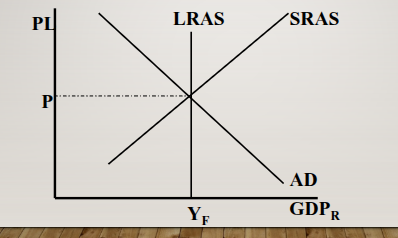
FULL EMPLOYMENT

Full Employment equilibrium exists where

AD intersects SRAS & LRAS simultaneously

RECESSIONARY GAP

when aggregate output is below potential output.

AKA: A recessionary gap exists when equilibrium occurs below full employment output (unemployment is above the nat. rate)

• to correct this, the government can increase spending, causing an increase in aggregate demand, which results in an increase in real GDP and income

• also, the government can decrease taxes to combat a recessionary gap, causing an increase in aggregate demand, which results in an increase in real GDP and income.

INFLATIONARY GAP

when aggregate output is above potential output.

AKA: An inflationary gap exists when equilibrium occurs beyond full employment output

CHANGES (Δ) IN AD (Consumption (C))

CHANGES (Δ) IN AD (Gross Private Investment (Ig)

CHANGES (Δ) IN AD (Government Spending (G))

CHANGES (Δ) IN AD (Δ Net Exports (Xn)

INCREASE IN AD

INCREASE IN AD

C↑, IG↑, G↑ and/or XN↑ .: AD → .: GDPR↑ & PL↑ .: u%↓ & π%↑

DECREASE IN AD

C↓, IG↓, G↓ and/or XN↓ .: AD ← .: GDPR↓ & PL↓ .: u%↑ & π%↓

CHANGES (Δ) IN SRAS (Input Prices)

CHANGES (Δ) IN SRAS (Productivity)

CHANGES (Δ) IN SRAS (Legal-Institutional Environment)

INCREASE IN SRAS

Input Prices↓, Productivity↑, and/or Deregulation

.: SRAS → .: GDPR↑ & PL↓ .: u%↓ & π%↓

DECREASE IN SRAS

Input Prices↑, Productivity↓, and/or Regulation

.: SRAS ←.: GDPR↓ & PL↑ .: u%↑ & π%↑

EQUILIBRIUM (in short and long run)

• in the short run, equilibrium may be above or below the full employment rate. In other words, AD and AS may not intersect at the LRAS.

• In the long run, equilibrium will be at the LRAS because, in the long run, AS will have adjusted so that short-run aggregate output is equal to the potential output

demand-pull inflation

Increases in AD cause the price level and the level of output and employment to rise

Demand Shocks

Decreases in AD cause the price level and the level of output and employment to fall

• increases or decreases in AD are known as Demand

  Shocks

• An event that shifts the aggregate demand curve is a

increases in AS have a positive effect on…

both price level and output

• When AS shifts right, price levels fall or stabilize, but output increases

Decreases in AS hurt both…

the price level and output

cost-push inflation or stagflation

combination of inflation and stagnating (or falling) aggregate output

• When AS shifts left, price levels rises and output falls.

• When AS shifts right, price levels fall and out put rising

supply shock

Any unexpected change in AS, whether positive or negative

SELF-CORRECTING NATURE OF ECONOMY (long run AS)

In the long-run aggregate supply will shift so that equilibrium will be at the long- run level of output

• This happens as nominal wages and other input prices adjust to meet the current price leve

AD-AS model

In the AD-AS model, the aggregate supply curve and the aggregate demand curve are used together to analyze economic fluctuations.

short-run macroeconomic equilibrium

The economy is in short-run macroeconomic equilibrium when the quantity of aggregate output supplied is equal to the quantity demanded.

short-run equilibrium aggregate price level

the aggregate price level in the short-run macroeconomic equilibrium

short-run equilibrium aggregate output

the quantity of aggregate output produced in the short-run macroeconomic equilibrium

long-run macroeconomic equilibrium

when the point of short-run macroeconomic equilibrium is on the long-run aggregate supply curve

output gap

the percentage difference between actual aggregate output and potential output.

self-correcting

The economy is self-correcting when shocks to aggregate demand affect aggregate output in the short run, but not the long run.

Stabilization policy

the use of government policy to reduce the severity of recessions and rein in excessively strong expansions

when does econom contract or expand (government)

When the government increases spending or transfer payments or decreases taxes (to give consumers more income), the economy expands. When the government decreases spending or transfer payments or increases taxes, the economy contracts.

Social insurance

programs are government programs intended to protect families against economic hardship.

Expansionary fiscal policy

increases aggregate demand

Contractionary fiscal policy

reduces aggregate demand

Lump-sum taxes

taxes that don't depend on the taxpayer's income

Automatic stabilizer

government spending and taxation rules that cause fiscal policy to be automatically expansionary when the economy contracts and automatically contractionary when the economy expands. (Fiscal policies adjust tax rates and transfer payments to stabilize the economy)

Discretionary fiscal policy

is fiscal policy that is the result of deliberate actions by policy makers rather than rules,

Fiscal Policy (recessionary gap)

government spending increases and taxes decrease (leads to AD increase)

Monetary Policy (recessionary gap)

reserve Ratio decreases, Discount rate decrease, or buy bonds (leads to an increase in the money supply which lowers interest rates which will increase AD)

No Policy or self correcting (recessionary gap)

wages will drop (SRAS will increase)

Fiscal Policy (Inflationary Gap)

government spending decreases, taxes increase (lead to AD decrease)