Paired sample t-test

t-Test uses 

Test variable must be continuous  

Paired / Dependent Samples t-Test 

Tests whether there is a statistically significant difference between two dependent sample means 

• Used when the SAME group is measured twice (e.g. before vs after) 

• Used when two groups are matched or paired on some basis 

• Design = within-subjects / dependent groups 

• IV = experimental condition with 2 levels 

• DV = continuous outcome (e.g. reaction time in milliseconds) 

Hypotheses and NHST 

• H₀: μ₁ = μ₂  →  μ₁ − μ₂ = 0 (no true mean difference) 

• Hₐ: μ₁ ≠ μ₂  →  μ₁ − μ₂ ≠ 0 (a true mean difference exists) 

• Set α = .05 

• p < .05 → reject H₀ → statistically significant difference 

• p ≥ .05 → do not reject H₀ → not statistically significant 

Paired t-Test assumptions 

• DV must be interval or ratio 

• Both sets of scores should be approx normally distributed 

• The DIFFERENCE SCORES should also be approx normally distributed 

Cohen’s d 

Measures the size of the difference between the two means in standard deviation units 

• Tells us practical significance / magnitude 

Cohen’s d - interpretation

Reading a Paired t-Test Result 

• Look at the two means first to identify the direction of the difference 

• Use the p value to decide statistical significance 

• Use the 95% CI of the MEAN DIFFERENCE: if it includes 0, the difference is not statistically significant at α = .05 

• Use Cohen’s d to describe practical significance 

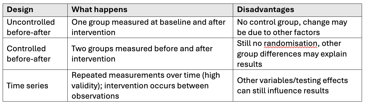
Quasi-Experimental Design 

Resembles an experimental design BUT there is no random allocation of participants into groups 

• Participants may self-select into groups or interventions may be assigned to pre-existing groups 

• Some have no control group 

• Used when: an RCT is not feasible, practical or ethical 

• Can support a relationship between an intervention/exposure and outcome 

- Lack of randomisation makes alternative explanations harder to rule out 

Quasi-Experimental Design - limitations

• Practice/testing effects 

• Changes in the data-collection instrument 

• Lack of control over other variables 

Types of Quasi-Experimental Design 

Internal validity 

Whether differences between study groups are due to the IV rather than confounding, bias or other explanations 

• Random chance: assess using p values and 95% CIs 

• Confounding: randomisation helps distribute differences between groups 

• Bias: blinding and placebo treatments can reduce systematic differences in data collection 

Random Error vs Systematic Error 

Selection Bias 

Sample differs systematically from the population 

• Under- or over-representation of particular groups 

• Systematic differences in how participants are recruited into study groups 

• Low response rate can produce a sample that does not accurately represent the target population 

Information Bias 

Systematic differences in data collection, measurement or classification 

Recall bias

Cases may remember previous exposures differently from controls 

Reporting bias

Participants under-report or exaggerate responses 

Recording bias

More info may be recorded for one group than another 

Interviewer bias

Questions/recording differ between participants 

Attrition/withdrawal bias

Loss to follow-up, especially if disproportionate between groups 

Misclassification bias

Participants systematically classified incorrectly (e.g. exposed/non-exposed or diseased/disease-free) 

Confounding 

Effect of the study factor/exposure on the outcome is mixed with the effect of another variable 

• Should be related to the exposure AND be an independent risk factor for the outcome/disease 

Ways to control confounding: 

• Randomisation: distributes differences between groups 

• Matching: controls matched to cases on factors such as age, sex or smoking 

• Stratified analysis: analyse separate subgroups (e.g. age groups, sex, smokers/non-smokers) 

Hierarchy of evidence