Biostats ch. 9
 Call Kai
 Learn
 Practice Test
 Spaced Repetition
 Match
 Flashcards
 Knowt Play
1/23

There's no tags or description
Looks like no tags are added yet.
24 Terms
Categorical data
Qualitative characteristics of individuals that do not have magnitude on a numerical scale.
a) Nominal (no inherent order)
b) Ordinal (inherent order)
Contingency analysis is how we see associations between categorical variables
Experimental Study
Experimental if the researcher assigns treatments randomly to individuals.

Often consists of randomized controlled trials (RCTs)

Observational Study
Observational if the assignment of treatments is not made by the researcher

Can be cross-sectional studies
Can mean, like in NHANES, that you have a different random sample for different years

Can be longitudal
Uses a longitudinal cohort
Longitudinal - follows same people through time
Cohort - sample has one characteristic
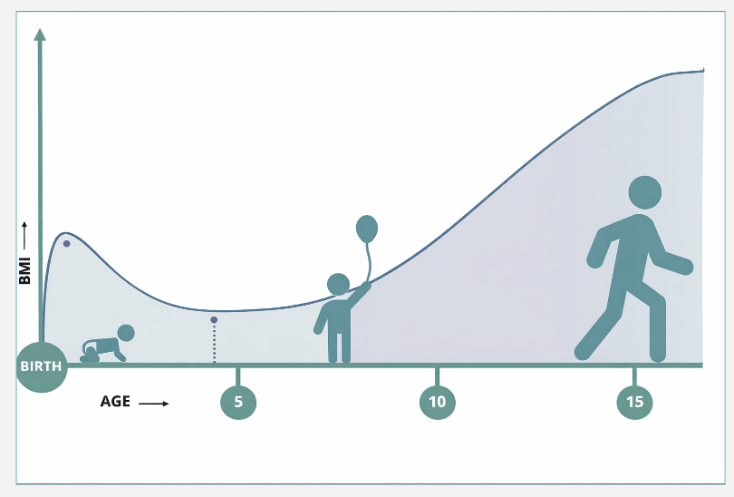
Can be a case-control study
2 groups
1) people who have the outcome
2) control group of people who don't have outcome
Helps you determine whether to use relative risk or odds
Identified by one group having the outcome and one not
Each row on the data set is a participant

Contingency analysis
Contingency analysis estimates and tests for an association between two or more categorical variables
It Determines the extent to which one variable is “contingent” on the other
2 variables (exposure and an outcome)
Binary answers (yes or no)

Examples:
Are smokers more likely to drink coffee than non-smokers?
Drink coffee (yes or no); smoke (yes or no)
Were men and women equally likely to survive the sinking of the Titanic?
sex (male or female); survive (yes or no)
2 × 2 contingency tables
Two categorical variables, each with two groups
Three different ways to analyze these data VARIABLES MUST BE CATEGORICAL TO APPLY THESE TESTS
Relative risk
Odds ratio
X² contingency test
Example:
Were men and women equally likely to survive the sinking of the Titanic?
sex (male or female); survive (yes or no)

2X2 contigency: Relative risk → LONGITUDAL STUDY + RCT
Relative risk is the probability of an undesired outcome in the treatment group divided by the probability of the same outcome in a control group

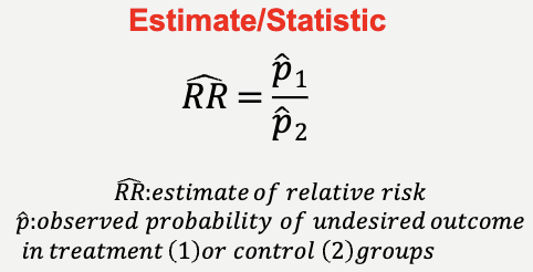

A ratio of 1 suggests no difference
Slightly higher means a slightly higher association (need to see confidence interval though)
If you get RR = 1.08 and this is in the confidence interval, then there is a slight association, but there is no statistical significance (find CI using log scale then convert back)
If 1 is your reference and you get RR = 2.5, you have 1.5x more risk
Based on exposure, must give result in relation to something (in this case exposure)
Don't need to present p-value because CI tells you you are pretty sure
When to apply relative risk
Relative Risk is the "gold standard" for:
Longitudinal Studies:
You start with a group of healthy people, divide them by exposure (e.g., smokers vs. non-smokers), and follow them forward in time.
Randomized Controlled Trials (RCTs):
You compare the risk of an outcome in the treatment group versus the control group.
Key Rule: You can only calculate RR if you know the incidence (the number of new cases) within a specific population.
Risk is a proportion:

Steps for relative risk, SE and confidence interval short cut method
1) Calculate the Relative Risk (RR)

2) Take the natural log of RR
ln(RR)
3) Calculate the standard error of ln(RR)
Using the a, b, c, d counts:

4) Build the 95% CI on the log scale

5) Exponentiate to return to the RR scale

Relative Risk Example Problem
Aspirin has been shown to reduce the risk of stroke and heart attack
Does it also reduce the risk of cancer?
10 year study in which 39,876 woman took either aspirin or placebo every other day


1) calculate the relative risk
2) calculate the SE
3) calculate the CI
4) conclusion based on RR
In medical studies, the convention is:
to calculate the odds of the outcome “diseased” or “died”
Set the control/placebo as group 2
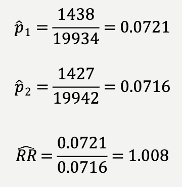
Method 1)

Method 2) Shortcut


2) Standard Error


3) Confidence interval

4) Conclusion based on relative risk
0.94 < RR < 1.08
Potential outcomes:
1: risk in two groups are equal
<1: risk in group 1 (numerator, treatment) is lower
>1: risk in group 1 (numerator, treatment) is higher
Range includes 1 (no difference in risk of getting cancer between aspirin and placebo groups)
Data are consistent with a small beneficial effect, a small deleterious effect, or no effect at all
Example of RR in a study
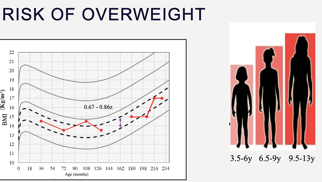

Usually, you expect children's weight to follow a trajectory
Movement in the channel was calculated using relative risk
1 = reference value (for comparison)
2, 3 = compared to the reference variable
Changing channels increased risk for deviation from normal weight
Relative Risk Practice Problem: School Lunches and Food Poisoning
After a school picnic, several students reported symptoms of food poisoning. A researcher conducted study to evaluate the association between eating the "Egg Salad" and the risk of getting sick.

1) Find RR
2) Find SE
3) Find CI
4) Conclusion based on RR



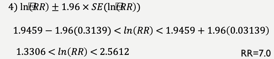


Students who ate the egg salad had a substantially higher risk of food poisoning compared with those who did not eat it (RR = 7.00; 95% CI: 3.78–12.95)
Relative Risk Practice Problem: Physical Activity and Heart Disease
A 10-year longitudinal study followed a group of sedentary adults and a group of active adults to determine the risk of developing Hypertension.

1) Find RR
2) Find SE
3) Find CI
4) Conclusion based on RR
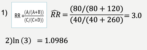


Sedentary adults had three times the risk of developing hypertension compared with physically active adults (RR = 3.00; 95% CI: 2.15–4.19)
2×2 Contingency: Odds Ratio → case-control study
The odds of success are the probability of success divided by the probability of failure

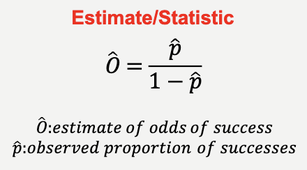
If O = 1 then the odds of success and failure are equal, thus no contingency between variables
The odds ratio is the odds of success in one group divided by the odds of success in a second group

Potential outcomes
1: odds of success in two groups are equal
<1: odds of success (disease) in group 1 (numerator, treatment) less likely
>1: odds of success in group 1 (numerator, treatment) more likely
SHORT CUT

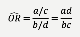
1st variable is exposed 2nd is unexposed → so you can compare exposed to unexposed
Steps for Odds ratio, SE and confidence interval short cut method
1) Calculate the odds ratio (OR)

2) Take the natural log of OR
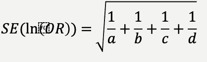
3) Calculate the standard error of ln(OR)
using the a, b, c, d counts
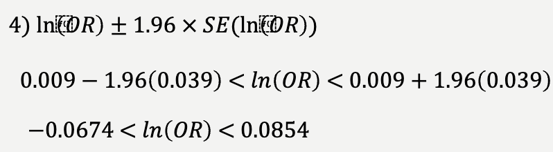
4) Build the 95% CI on the log scale

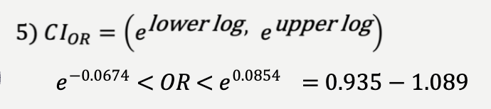
5) Exponentiate to return to the OR scale

When to apply odds ratio
Case–control studies
To identify: You will always have a group with the outcome and another matching group that does not have the outcome
Cross-sectional (rare outcome < ~10%)
Logistic regression models (binary, ordinal, or multinomial)
Binary (yes, no)
Ordinal (there is an order, ex. high, middle, low) → strongly agree, agree, disagree
Multinomial (many categories with no order)
Odds ratio example
Aspirin has been shown to reduce the risk of stroke and heart attack
Does it also reduce the risk of cancer?
10 year study in which 39,876 woman took either aspirin or placebo every other day
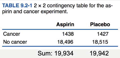
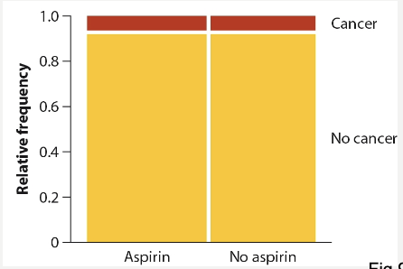
1) Calculate the odds of success
2) Calculate odds ratio (are they significant)
3) Use the short cut method to find the same thing
Method 1)

Odds of developing cancer for aspirin group
O1 = 0.0777
Odds of developing cancer in no aspirin (placebo) group
O2 = 0.0771
Are these statistically different?


>1: odds of success in group 1 (numerator, treatment) more likely
Method 2) Short cut


2)

3)

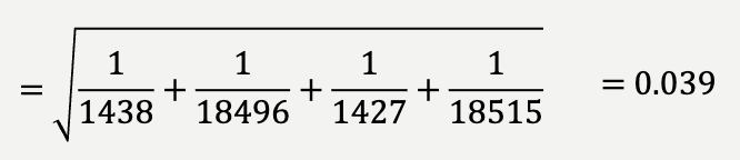
4)
5)
Conclusion:
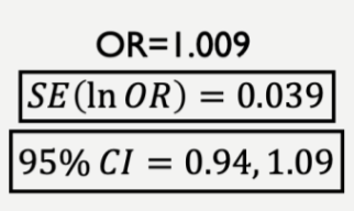
95% confident that OR is between 0.94 and 1.09
Range includes 1 (no difference in odds of getting cancer between aspirin and placebo groups)
Data are consistent with a small beneficial effect, a small deleterious effect, or no effect at all
Example of odds ratio data
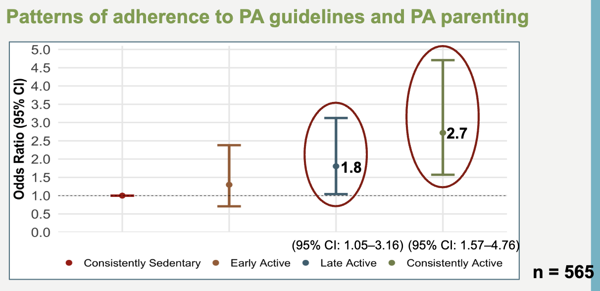
Odds ratio: have something you are comparing
The reference category (sedentary) is 1, which you are comparing other categories to
Example Problem: Odds ratio Vaping and Acute Lung Injury
Doctors at a city hospital identified 40 patients with a specific lung injury (Cases). They also selected 80 patients of the same age who were at the hospital for unrelated reasons (Controls). The researchers looked backward to see how many in each group had a history of vaping.

1) Create a table
2) Calculate OR
3) Is the OR significant

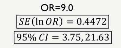
OR = 9 means positive association → is it significant? Can't say because we don't know the CI or P-value
Need to know p-value or OR CI in order to confirm
When using R, the p-value is easiest to find



Conclusion:
People with a history of vaping had 9 times the odds of lung injury compared to those who did not vape (OR = 9.00; 95% CI: 3.75–21.63).
Example Problem: Odds ratio Sleep Deprivation and Car Accidents
A researcher investigates the link between sleep and accidents. They find 100 drivers involved in a crash last night (Cases) and 100 drivers who were on the road but did not crash (Controls). They interviewed them to find out who slept less than 6 hours.

1) Create a table
2) Calculate OR
3) Is the OR significant


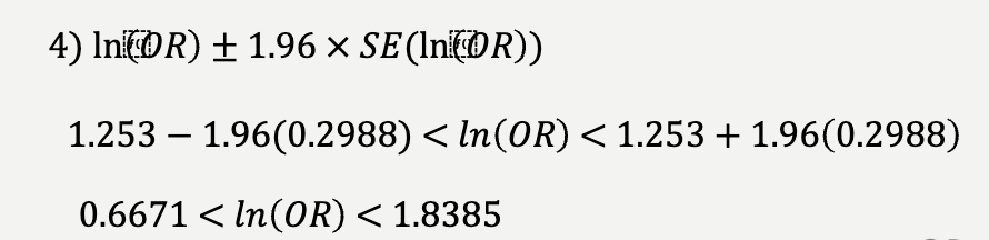


Conclusion:
Drivers who slept less than 6 hours had 3.5 times the odds of being involved in an accident compared with those who slept more than 6 hours (OR = 3.50; 95% CI: 1.95–6.29)
X² contingency test
The X² contingency test is used to test the association between two categorical variables
Special case of the X² goodness-of-fit test where the null model is independence of variables
Same assumptions of X² goodness-of-fit test
No cells have expected frequency less than one
No more than 20% of cells have expected frequency less than five
If these assumptions are not met, then you can use Fisher’s exact test
For an X^2 test with 2 variables
Framing = H0 : independent, HA: associated
Compare our X^2 to the table X^2
If our value is larger, we reject H0 → so there is an association
If there are more than two categories in your variable → use X^2 test
X² contingency Test Steps
Find H0 (independent) and HA (associated)
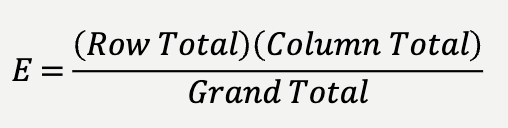
Calculate expected frequencies from observed data
If the variables are independent, expected frequencies are calculated as:

Calculate X²

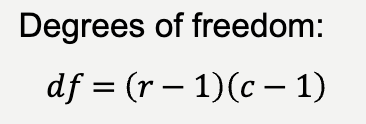
Find degrees of freedom

r = number of rows
c = number of columns
compare our X² with critcal value and df
if our value is larger than critical value we reject H0
Example Problem: X² contingency test
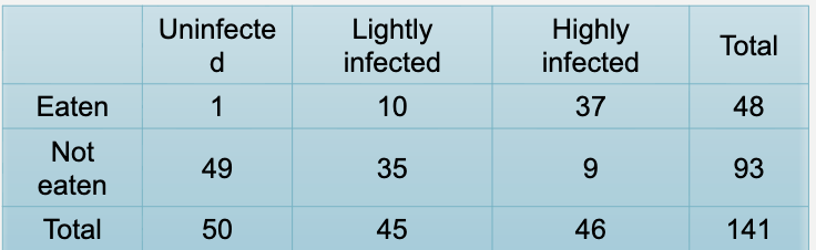
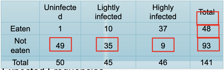
Testing the association between two categorical variables: Infection level and predation risk in fish
Research Question: Is the probability of being eaten by birds associated with the level of parasite infection?
Variables:
Infection level (Uninfected, Lightly infected, Highly infected)
Outcome (Eaten, Not eaten)
1) H0 and HA?
2) Expected frequencies
3) Calculate X²
4) Df
5) Critical value and decision
1)
Null hypothesis (H₀): Infection level and predation are independent.
Alternative hypothesis (HA): Infection level and predation are associated.
2)


3)


X² = 69.48
4)


5)


Decision:
Since 69.48 >5.99, We reject H0.
There is a significant association between infection level and predation. Predation rates increase with parasite infection:
• Uninfected: 2% eaten
• Lightly infected: 22% eaten
• Highly infected: 80% eaten

Example Problem: X² contingency test Exercise and Sleep Quality
A researcher wants to know whether exercise is associated with sleep quality.

1) H0 and HA?
2) Expected frequencies
3) Calculate X²
4) Df
5) Critical value and decision
Null hypothesis (H₀): Exercise and sleep quality are independent.
Alternative hypothesis (HA): Exercise and sleep quality are associated.


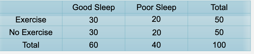


X² = 16.66


Conclusion:
Since 16.66 >3.84, We reject H0
There is a significant association between exercise and sleep quality. People who exercise are more likely to report good sleep.
Exercise: 80% reported good sleep
No exercise: 40% reported good sleep
Example Problem: X² contingency test Coffee Consumption and Headaches
A researcher wants to know whether coffee consumption is associated with headaches.

1) H0 and HA?
2) Expected frequencies
3) Calculate X²
4) Df
5) Critical value and decision
Null hypothesis (H₀): Coffee intake and headaches are independent.
Alternative hypothesis (HA): Coffee intake and headaches are associated


X² = 22.10
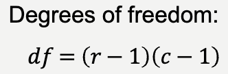



Since 22.10 >5.99, We reject H0.
There is a significant association between coffee consumption and headaches. People who consume more coffee are more likely to report headaches.
Low coffee intake: 16% reported headaches
Moderate coffee intake: 30% reported headaches
High coffee intake: 60% reported headaches