Comparing Distributions

In each of (1) and (2), two viewpoints are presented.

Choose a statistic that will help you decide between viewpoints.

Data: the results of 400 tosses of a coin

(1)

• “This coin is fair.”

• “No, it’s not.”

(2)

• “This coin is fair.”

• “No, it’s biased towards heads.”

*the statistic you choose depends on what the second viewpoint is claiming

(1) very large or very small values of the percent of heads suggest “not fair”

• the distance between percent of heads and 50% is key

• Statistic: | percent of heads - 50% |

• large values of the statistic suggest “not fair”

(2) Large values of the percent of heads suggest “biased towards heads”

• statistic: percent of heads (or percent of heads - 50%)

“Fair”

For both (1) and (2)

• the percent of heads in the 400 possess is a good starting point, but might need adjustment

• A percent of heads around 50% suggest “fair”

Distance Between Disributions

• people on the panels are of multiple ethnicities

• Distribution of ethnicities is categorical

• to see whether the distribution of ethnicities of the panels is “close: to that of the eligible jurors, we have to measure the “distance” between two categories

Total Variation Distance

Every distance has a computational recipe

Total Variation Distance (TVD):

• for each category, compute the difference in proportions between two distributions

• take the absolute value of each difference

• sum and then divide by 2

Summary of Method

To assess whether a sample was drawn randomly from a known categorical distribution:

• Choose TVD as the statistic because it measures the distance between categorical distributions

• Simulate: sample at random from the population and compute the TVD from the random sample: repeat numerous times

• Compute:

  • empirical distribution of simulates TVDs

  • Actual TVD from the sample in study

Comparison with panels Selected at Random: ex: Panels in Alameda County

Question: What if we selected at random sample of 1,453 people from the population of eligible jurors? Will the distribution of their ethnicities look like the distribution of panels

We can answer this question by using sample_proportions and augment the jury table with a column of the proportions in our sample.

We will sample with replacement (because when the size of a sample is small relative to the size of the population, sampling without replacement resembles sampling with replacement)

eligible_population = jury.column(‘Eligible’)

sample_distribution = sample_proportion(1453, eligible_population)

panels_and_sample = jury.with_column(‘Random Sample’, sample_distribution)

panels_and_sample

In the cell above, we sample at random 1453 times from the distribution of eligible jurors, and display the distribution of the random sample along with the distribution of the eligible and the panel in the data

The bar chart shows that the distribution of the random sample resembles the eligible population but the distribution of the panels does not.

To assess whether this observation is particular to one random sample or more general, we can simulate multiple panels under the model of random selection and see what the simulation predicts. But we won’t be able to look at thousand of bar charts. We need a statistic that will help us assess whether or not the model or random selection supports the data

Continued: A New Statistic: The Distance between Two Distributions

Now we have to quantify the distance between two distributions

For this we will compute a quantity called the total variation distribution. The calculation is an extension of how we find the distance between two numbers

First: find the difference between the two proportions in each category

#Augment the table with a column of differences between proportions

Jury_with_diff = jury.with_column (‘Absolute Difference’, np.abs( jury.column(‘panels’) - jury.column(‘Eligible’) )

Second:

jury_with_diffs.column('Absolute Difference').sum() / 2

Output:

0.14

Meaning: The quantity 0.14 is the total variation distance (TVD) between the distribution of ethnicities in the eligible juror population and the distribution in the panel

In general, the TVD between two distributions measure how close the distributions are. Therefore, the larger the TVD, the more different the two distributions appear.

We will see the total variation distance distribution as the statistic to simulate under the assumption of random selection. Large values of the distance will be evidence against random selection

Continued: Simulating the Statistic Under the Model

To see how the TVD varies across random samples, we will simulate it repeatedly under the model of random selection from the eligible population.

Let’s organize our calculation. Since we are going to be computing total variation distance repeatedly, we will write a function that computes it for two given distributions

The function total_variation_distance takes two arrays containing the distribution to compare and returns the TVD between them

def total_variation_distance(distribution_1, distribution_2) 
    return sum(np.abs(distribution_1 - distribution_2)) / 2

This function will help us calculate our statistic in each repetition of the simulation.

total_variation_distance(jury.column('Panels'), jury.column('Eligible'))

Output:

0.14

Next:

we will use the function to compute the TVD between the distribution of eligible jurors and one random sample.

Recall eligible _proportions is an array containing the distribution of the eligible jurors, and that our sample size is 1453

In the first line, we will use sample_proportion to generate a random sample from the eligible proportion. In the next line we will use total_variation_distribution to compute the TVD between the distribution in the random sample and the eligible population

sample_distribution = sample_proportions(1453, eligible_population
iStotal_variation_distance(sample_distribution, eligible_population)

Simulatinf One Value of the Statistic

Lets define a function one_simulated_tvd that returns one simulates value of the TVD under the hypothesis of random selection

# Simulate one simulated value of 
# the total variation distance between
# the distribution of a sample selected at random
# and the distribution of the eligible population

def one_simulated_tvd():
    sample_distribution = sample_proportions(1453, eligible_population)
    return total_variation_distance(sample_distribution, eligible_population)  

Simulatinf Multiple Values

Now we can apply the familiar process of using a for loop to create an array consisting of 5000 such difference

tvds = make-array()

repetitions = 5000

for i in np.arange(repetition)

tvds = np.append(tvds, one_simulated_tvd())

Assessing the Model of Random Selection

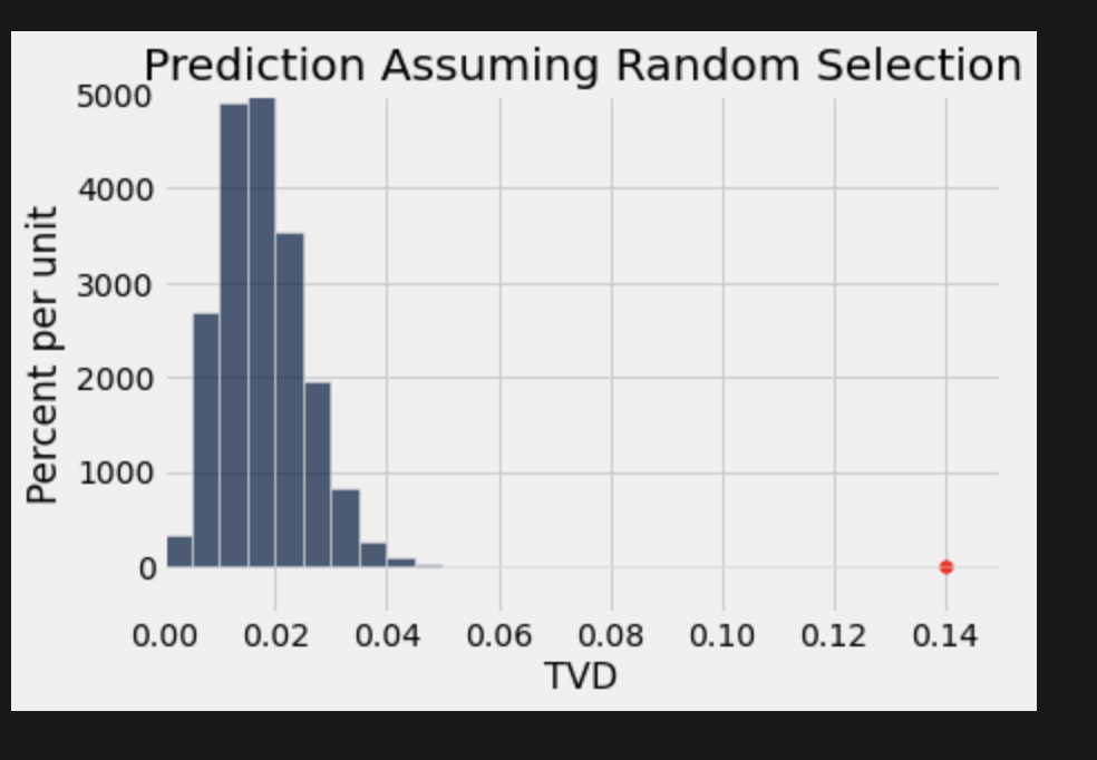
Here is the empirical histogram of the simulated distances. it shows that if you draw 1453 panelists at random from the pool of eligible candidates, then the distance between the distributions of the panelists and the eligible population is rarely more than about 0.05

The panelist in the study, however, were not quite so similar to the eligible population. The total variation distance between the panels and the population was 0.14, shown, as the red dot on the horizontal axis. It is far beyond the tail of the histogram and does not at all like a typical distance between the distribution of a random sample and the eligible population

The simulation shows that the composition of the panel in the ACLU study is not consistent with the model of random selection. Our analysis support the ACLU’s conclusion that the panels were not representative of the distribution provided for the eligible jurors