Genetics and Molecular Biology: Chromosomes, Gene Regulation, and Functional Genomics

Comprehensive vocabulary flashcards covering chromosomal aneuploidies and aberrations, forward and reverse genetics, prokaryotic and eukaryotic gene regulation, epigenetics, genomic imprinting, and functional genomics sequencing methods.

Karyotype

The complete chromosomal complement of an individual organism or cell, arranged and displayed systematically from a mitotic metaphase spread according to chromosome size and morphology.

Euploidy

A condition in which a cell or organism possesses an exact multiple of the normal, standard chromosomal set characteristic of its species.

Aneuploidy

A chromosomal condition in which one or more specific individual chromosomes are either missing or present in excess, resulting in an abnormal chromosomal ratio.

Trisomy

The presence of an extra copy of an individual chromosome ($2n + 1$), representing a prominent feature of spontaneously aborted human fetuses due to altered gene expression disrupting normal development.

• Trisomies show up all over the miscarriage column (16, 22, 15, 21, 14, and so on). They are a prominent feature of spontaneously aborted fetuses because extra gene dosage disrupts normal development.

• In live births, only a few trisomies appear: 13 (17), 18 (13), and 21 (113). These are among the smallest chromosomes, so they carry fewer genes, so the imbalance is less catastrophic.

• Look at the red arrows for trisomy 21: 350 miscarriages vs 113 live births. About 113/(350+113) ≈ 24% survive to birth. Trisomy 21 is the most common viable autosomal trisomy, but even it is mostly lost.

Monosomy

The absence of one copy of a homologous chromosome pair ($2n - 1$); among viable human fetuses, it is observed only for the $X$ chromosome ($45,XO$).

• No autosomal monosomy is viable. The only viable monosomy is X (the blue arrows: XO, Turner syndrome).

• Even so, XO is very harsh: 1,350 in miscarriages vs only 8 live births. About 99% are lost.

Sex chromosome trisomies (XXY, XYY, XXX) are common among live births (44-46 per 100,000) and rarely miscarried. That’s because extra X’s are mostly inactivated (slide 6) and the Y has very few genes.

Why can the X tolerate aneuploidy but autosomes can’t? The X has a built-in way of balancing its dosage (X-inactivation), and the Y is gene-poor. Autosomes have no such mechanism, so any change in dosage hits fully. This sets up everything on slides 5-9.

The table also lists translocations and polyploidy. Triploid (3n) and tetraploid (4n) are common in miscarriages and absent in live births. Balanced translocations are common in live births (164) because they’re harmless, while unbalanced ones are mostly lost (225 miscarried vs 52 live). That’s a preview of the later slides.

Barr Body

A condensed, cytologically visible, transcriptionally inactive $X$ chromosome positioned at the nuclear periphery of female mammalian somatic cells.

Dosage Compensation

The mechanism that equalizes the expression of $X$-linked genes between males ($XY$) and females ($XX$), mediated in mammals by random early embryonic inactivation of one $X$ chromosome in each cell lineage.

Paracentric Inversion

A chromosomal inversion that does not include the centromere; crossing over inside its inversion loop during meiosis generates a dicentric chromosome and an acentric fragment, resulting in inviable recombinant gametes and suppressed recombination.

Pericentric Inversion

A chromosomal inversion that includes the centromere; crossing over within the inversion loop generates unbalanced recombinant products with large duplications and deletions, resulting in inviable gametes.

Tandem Duplication

A chromosomal structural alteration where an identical chromosome segment is repeated adjacent to the original segment in the same orientation, making the region prone to unequal crossing over during meiosis.

Robertsonian Translocation

A non-reciprocal translocation involving the fusion of two acrocentric chromosomes near their centromeres, such as translocations involving Chromosome $21$ that cause familial Down syndrome.

A Robertsonian translocation forms when two chromosomes (typically two acrocentrics such as 14 and 21) fuse at their centromeres. The tiny short arms are lost, but they carry mostly redundant genes, so the carrier is unaffected. This is called “T” on the slide.

Notation on the slide: “N” is a normal chromosome (the one that fused with 21, e.g. 14), “21” is a normal chromosome 21, and “T” is the fusion.

• Unaffected carrier: N T 21. He or she has one normal N, one fusion T (which contains one N-worth and one 21-worth of material), and one free 21. In total there are two doses of each, so everything is balanced.

• Normal partner: N N 21 21.

The slide shows three possible kids:

• N N 21 21: a normal karyotype, unaffected.

• T N 21 21: Down syndrome. The child has T (carrying a 21) + two free 21’s = three doses of chromosome 21, even though the chromosome count is only 46.

• T N N 21: inviable. Three doses of the other chromosome (trisomy N).

(Others are possible, such as a balanced carrier child, and the monosomies, which also die.)

Familial Down syndrome vs. trisomy 21 due to nondisjunction:

• Nondisjunction: a random error in meiosis. It occurs sporadically, and risk goes up with maternal age. The child has 47 chromosomes with a free extra 21.

• Translocation (familial): inherited from a balanced carrier parent. It runs in families and isn’t tied to maternal age. The child has 46 chromosomes with the extra 21 attached to another chromosome.

Single Nucleotide Polymorphism (SNP)

A specific position in the genome where different individuals carry different single nucleotide base pairs; represents the most common type of genetic variation in humans.

Short Tandem Repeat (STR)

A DNA marker consisting of short, repeating tandem nucleotide units ($2$ to $6\text{ bp}$) at specific genomic loci that vary in repeat count among individuals, providing the basis for forensic DNA fingerprinting.

Forward Genetics

A genetic approach that begins with identifying individuals exhibiting a variant mutant phenotype of interest and works backward to identify the specific causative gene and mutation.

Autophagy

A conserved eukaryotic degradation and recycling process wherein cellular components are enveloped in double-membrane vesicles and delivered to the vacuole or lysosome to sustain viability under starvation conditions.

Genetic Screen

An experimental approach in which a mutagenized population of organisms is individually tested or visualised to discover rare individuals displaying a specific phenotype of interest.

Slide 10: Survival graph

Axes: y = % viable cells (scale 10, 50, 100), x = days of nitrogen starvation (0-5).

• Wild type (open circles): stays flat near ~100%. Starved wild-type cells survive.

• Mutant (filled circles): stays near 100% for the first ~2 days, then drops: ~55% at day 3, ~30% at day 4, ~20% at day 5.

Meaning: the mutant can’t survive starvation. It lacks something the wild type has. The first couple of days look fine because the cells still have reserves. The deficit only shows once those run out.

Slide 11: Microscope images

• Wild type (left): after starvation, the vacuole contains a cluster of round bodies (the arrow). Autophagosomes accumulate.

• Mutant (right): the vacuole is a large, empty-looking white space. Autophagosomes do not accumulate.

Genetic Selection

An experimental technique where organisms are placed under environmental growth conditions that kill wild-type individuals while allowing only mutants with a specific survival trait (such as drug resistance) to form colonies.

Ascus

A specialized sac in budding yeast (Saccharomyces cerevisiae) that encases the four haploid spore products of a single meiotic division, known as a meiotic tetrad.

Complementation Test

A genetic test in which two recessive mutants with the same phenotype are crossed; production of wild-type progeny indicates mutations in different genes, whereas production of mutant progeny indicates alleles of the same gene.

Reverse Genetics

An experimental strategy that begins with a known DNA sequence or gene of interest, disrupts or modifies that sequence directly, and evaluates the resulting organismal phenotype to determine gene function.

Homology-Directed Repair (HDR)

A high-fidelity DNA double-strand break repair pathway that requires a homologous donor template DNA sequence to guide accurate repair via strand invasion.

Non-Homologous End Joining (NHEJ)

An error-prone DNA double-strand break repair pathway that ligates broken DNA ends directly together without requiring a homologous template, frequently causing small insertion or deletion mutations (indels).

Cas9 Nuclease

A bacterial endonuclease adapted from CRISPR adaptive immunity systems that complexes with a single guide RNA (sgRNA) to bind and introduce a double-strand break at a specific target DNA site.

Protospacer Adjacent Motif (PAM)

A short sequence motif ($5'\text{-NGG-3'}$ in Streptococcus pyogenes Cas9) situated directly adjacent to the non-complementary strand of the target sequence that is required for Cas9 DNA binding and cleavage.

Cre-lox System

A site-specific recombination technology wherein Cre recombinase catalyzes DNA excision between pair-wise $loxP$ target sites, commonly used to create tissue-specific or conditional gene knockouts in mice.

RNA-seq

A functional genomics method that isolates cellular RNA, enriches polyadenylated mRNA with oligo-dT beads, converts it to cDNA, and sequences it at high throughput to quantify gene expression and delineate exon boundaries.

Bisulfite Sequencing

A technique that maps cytosine methylation across the genome by treating DNA with sodium bisulfite, which selectively deaminates unmethylated cytosines into uracils while preserving $5$-methylcytosines intact.

ChIP-seq

Chromatin Immunoprecipitation sequencing; a method that uses formaldehyde crosslinking, chromatin fragmentation, and specific antibodies to isolate and sequence DNA fragments bound by a transcription factor or modified histone.

ATAC-seq

Assay for Transposase-Accessible Chromatin with sequencing; uses a hyperactive $Tn5$ transposase to simultaneously cleave accessible DNA and insert sequencing adapters to identify open chromatin and active regulatory regions.

Hi-C

A genome-wide chromosome conformation capture method that pairs spatial crosslinking with restriction enzyme digestion, biotin labeling, and ligation to map three-dimensional genomic interactions and Topologically Associating Domains.

Topologically Associating Domains (TADs)

Three-dimensional structural domains of chromatin within chromosomes where internal regulatory interactions occur frequently, while interactions with elements in neighboring domains are constrained.

Cis-acting Element

A non-protein-coding DNA sequence (such as an operator, promoter, or enhancer) that regulates the expression of adjacent genes situated exclusively on the same chromosome or DNA molecule.

Trans-acting Factor

A diffusible regulatory molecule (typically a protein or RNA) encoded by a distinct gene that diffuses throughout the nucleus or cytoplasm to bind target cis-regulatory elements located on any DNA molecule.

Operon

A coordinated cluster of contiguous prokaryotic structural genes under the transcriptional control of a shared single promoter and operator, yielding a single polycistronic mRNA transcript.

Polycistronic mRNA

A continuous messenger RNA transcript found predominantly in bacteria that contains multiple distinct open reading frames ($\text{ORFs}$) translated independently into different polypeptides.

Negative Regulation

A transcriptional regulatory mechanism in which transcription is constitutively active by default and is turned off or blocked when a repressor protein binds to a specific operator sequence.

Positive Regulation

A transcriptional regulatory mechanism in which transcription is inherently inactive by default and requires the binding of an activator protein to the promoter or upstream regulatory site to stimulate transcription.

cAMP Receptor Protein (CRP)

A bacterial transcriptional activator that binds cyclic AMP ($\text{cAMP}$) during glucose starvation and binds the $lac$ operon promoter region to stimulate RNA polymerase binding and transcription initiation.

Super-Repressor ($lacI^S$)

A gain-of-function mutant allele of the $lacI$ gene encoding a repressor protein that can no longer bind the inducer (lactose), remaining permanently bound to the operator and causing uninducible, dominant repression in both cis and trans.

The normal repressor

• Binds the operator → operon OFF.

• When lactose shows up, lactose binds the repressor → repressor lets go → operon ON.

The repressor has two jobs: grab the operator, and respond to lactose by letting go.

What I^S is

A mutation in the lacI gene that breaks the second job only. The mutant repressor:

• Still binds the operator (works fine).

• Can’t bind lactose, so it never gets the “let go” signal.

So it stays stuck on the operator even when lactose is present. The operon can never turn on, which makes it uninducible. (“S” = super, because it’s a repressor that can’t be turned off.)

Why it’s gain-of-function

It isn’t a broken repressor (that would be I⁻, which makes the operon constitutive). It’s a repressor that’s too good: it holds on harder than it should. It gained an abnormal ability to stay bound.

trp Operon

A repressible bacterial operon whose expression of tryptophan biosynthetic enzymes is active in low tryptophan conditions and repressed when high tryptophan levels allow tryptophan to act as a corepressor with the aporepressor.

Upstream Activation Sequence (UAS)

A cis-acting regulatory DNA sequence located upstream of eukaryotic promoters (such as the yeast $GAL$ genes) that functions similarly to an enhancer by binding transcriptional activator proteins.

Gal4p

A yeast zinc-finger transcriptional activator that binds as a homodimer to Upstream Activation Sequences ($\text{UAS}$) to recruit RNA polymerase II and initiate transcription of the $GAL1$, $GAL7$, and $GAL10$ genes.

Gal80p

A eukaryotic co-repressor protein that binds directly to the activation domain of Gal4p to prevent transcription machinery recruitment in the absence of galactose.

Gal3p

A yeast cytoplasmic sensor protein that binds galactose and ATP to bind and sequester Gal80p, freeing the Gal4p activation domain to recruit RNA polymerase II.

Enhancer

A cis-acting DNA regulatory sequence that binds activator proteins to dramatically stimulate transcription of a target gene, operating independently of distance, relative orientation, or placement (upstream, downstream, or within introns).

Insulator Element

A specialized DNA sequence that limits the range of an enhancer by preventing it from interacting with inappropriate neighboring promoters, thus partitioning the genome into independent regulatory domains.

SWI/SNF Complex

A multi-subunit chromatin remodeling complex that uses ATP hydrolysis to alter nucleosome positioning and destabilize chromatin structure, exposing promoter regions to the transcription machinery.

CpG Island

A genomic DNA sequence rich in cytosine-guanine dinucleotide repeats, often located near gene promoters; dense methylation of its cytosines results in stable, heritable epigenetic transcriptional silencing.

Maintenance Methylase (DNMT1)

A specialized DNA methyltransferase that targets hemi-methylated CpG sites during DNA replication to add a methyl group to the newly synthesized strand, preserving epigenetic marks across somatic cell divisions.

Genomic Imprinting

An epigenetic modification phenomenon where a gene's expression depends on whether it was inherited from the mother or the father, established by parent-of-origin specific DNA methylation during gametogenesis.

Prader-Willi Syndrome

A human congenital disorder causing hyperphagia, severe obesity, and cognitive impairment, resulting from the inheritance of a paternal chromosome $15q11\text{-}q13$ deletion where the paternal copy of the $SNURF/\text{snoRNA}$ cluster is lost while the maternal copy remains silenced by imprinting.

Angelman Syndrome

A neurodevelopmental disorder causing severe developmental delay, motor ataxia, seizures, and inappropriate laughter, resulting from the inheritance of a maternal chromosome $15q11\text{-}q13$ deletion causing loss of maternal $UBE3A$ expression while the paternal allele is silenced by imprinting.

Tagmentation

An enzymatic workflow used in next-generation sequencing library preparation wherein hyperactive transposomes simultaneously fragment double-stranded genomic DNA and ligate synthetic sequencing adapters to the ends.

Shotgun Sequencing

A genome sequencing approach in which high-molecular-weight DNA is sheared into millions of random overlapping short fragments, sequenced in parallel, and computationally assembled into full-length genomic contigs based on sequence overlaps.

Aneuploidy effects meiotic segregation: meiosis yields two haploid (n) gametes and two disomic (n+1) gametes

Take a trisomic individual with 3 copies of one chromosome. In prophase I, homologs normally pair as 2 (a bivalent). With 3 you have two options:

Possibility 1: a trivalent. All three pair up together. At anaphase I, 2 go to one pole and 1 goes to the other. Any of the three pairings is possible.

Possibility 2: a bivalent + a univalent. Two pair normally. The third has no partner and goes to a random pole, so it can go with either member of the pair.

Either way, the result is the same. Two gametes get 1 copy (n, normal haploid). Two gametes get 2 copies (n+1, disomic). So half of a trisomic’s gametes carry the extra chromosome.

Bonus (the kind of question that could show up). Suppose the three chromosomes are A, A, and a. They’re all distinct physical chromosomes. Randomly pairing them gives:

• A₁A₂ pair, a alone → gametes AA and a

• A₁a pair, A₂ alone → gametes Aa and A

• A₂a pair, A₁ alone → gametes Aa and A

Total: 6 gametes, so 1 AA : 2 Aa : 2 A : 1 a (out of 6). The principle is: pick which two of the three go together, and the third goes the other way.

X - inactivation

If both X chromosomes were fully active in females, they’d make twice as much X-gene product as males. Mammals fix this by silencing one X in each cell of a female.

• Timeline: The zygote starts with both X’s active through early cleavage divisions. Somewhat later, each cell randomly picks one X to inactivate.

• Random: In each cell it’s a coin flip, paternal X or maternal X.

• Heritable by mitosis: Once a cell has inactivated a particular X, all of its descendants keep that same X off. The inactive state is copied through cell division.

• Barr body: The inactive X is condensed into a dense blob in the nucleus (the arrow in the micrograph).

• Result: A female is a mosaic. Some patches of tissue have X₁ on / X₂ off, and others have X₁ off / X₂ on.

A useful rule: # of Barr bodies = # of X chromosomes − 1. So XX has 1, XXX has 2, XXY has 1, XO has 0, and a normal XY male has 0. This ties back to slide 3, where the extra X’s of XXX and XXY are silenced, which is why those people are viable.

Small caveat: a few X genes escape inactivation (for example, genes in the region the X shares with the Y). That’s why XO and XXY people still have a phenotype even though dosage is mostly compensated.

pseudoautosomal regions

The regions of the X and Y chromosomes that share homology and undergo recombination during meiosis, allowing pairing between the X and Y chromosomes in males.

• The X and Y aren’t totally different. They share small matching regions (the pseudoautosomal regions) that carry the same genes on both chromosomes. Since the Y has these genes, males already have 2 copies of them. Natural selection therefore had no reason to silence them on the X, because silencing would give females only 1 dose and males 2. They escape inactivation, so females also get 2.

• The “dosage compensated” system only works properly for a normal XX or XY person. Change the chromosome number and the escapees throw off the balance:

  • XO (Turner syndrome): Only one X, and there’s no second X or Y to supply the second copy. So escapee genes are made at 1 dose instead of 2. Inactivation can’t fix that, because there’s nothing inactivated to begin with (0 Barr bodies).

  • XXY (Klinefelter syndrome): Two X’s, so one gets inactivated (1 Barr body). But the escapee genes on the inactive X are still active, so escapee genes are at 3 doses instead of 2 (two X’s plus the Y).

  In both cases, the escapee genes are the ones with the wrong dosage. That’s why XO and XXY people still have a phenotype, even though X-inactivation handled most of the X.

Human pedigree, manifesting carriers

Dad is XᴴY (unaffected). Mom, Betty, is XᴴXʰ (a carrier). Their kids:

• Jim: XʰY. A male with one X, so he has the disease. Normal.

• Nora: XʰXᴴ. A carrier, but she shows the trait.

Normally a heterozygous female for an X-linked recessive is unaffected, because her good allele covers. But because of mosaicism, her cells are a patchwork. By chance, if a large share of the relevant cells inactivated the good Xᴴ, then most active cells are running Xʰ. She’s a manifesting carrier (this is called skewed X-inactivation). The slide notes that up to 10% of carrier females may show the trait.

The other half of the title: for X-linked dominant traits, a heterozygous female has a milder version, because only some of her cells express the mutant allele, whereas a male has it in every cell.

Test takeaway: “Can a heterozygous female show an X-linked recessive trait?” Yes, via random/skewed X-inactivation. Don’t answer with a flat “no.”

Genetic vs. epigenetic

• Genetic: two individuals (or cells) differ in phenotype because their genotypes differ. Heritable through mitosis and meiosis.

• Epigenetic: two individuals (or cells) differ in phenotype because of a regulatory modification (not a DNA sequence difference). Heritable through mitosis.

Which describes X-inactivation? Epigenetic. The orange cells and the black cells in the cat have the identical DNA. They differ in which X is silenced (through chromatin condensation and chemical marks on the DNA/histones), and that silenced state is copied through mitosis. The sequence of the DNA itself hasn’t changed.

Holliday junction

A Holliday junction is a four-stranded, cross-shaped DNA intermediate that forms during genetic recombination and DNA repair. [1, 2, 3]

Key Features

• Structure: It consists of four double-stranded DNA arms joined together at a central exchange point.

Flanking markers

The deletion is in the middle (cde). The flanking markers are the ones on either side of it (A-B on the left, F-G on the right). The slide says these markers recombine less than normal. Two reasons:

1. Less DNA to cross over in. Crossovers happen at random spots along the DNA. If a chunk of the chromosome is missing, there are fewer places for a crossover to land between the flanking markers.

2. The deletion gets in the way of the crossover process.

   • The normal chromosome has cde, but the deleted one doesn’t. That region can’t line up, so pairing is messy right there.

   • A crossover creates a Holliday junction, where two DNA strands cross over, and it normally slides along the DNA (branch migration). Sliding only works where both chromosomes have matching sequence. At the deletion there is nothing to match, so the junction gets stuck.

number of recombinants relate to genetic distance

Crossovers land at random spots along a chromosome, roughly evenly spread. Picture the chromosome as a road and a crossover as a random “cut” somewhere on it.

• Two genes far apart: there’s a lot of road between them, so a random cut lands between them often. The genes get separated often, so you get many recombinants.

• Two genes close together: there’s very little road between them, so a random cut rarely lands between them. The genes almost always stay together, so you get few recombinants.

So the more recombinants you see, the more DNA must be sitting between the two genes. Recombinant frequency is a measurement of how much space is between them.

Inversions

Without a crossover inside the inversion, all four meiotic products are normal in gene content, so the inversion simply segregates as if it were a single allele: 1 WT : 1 WT : 1 Inv : 1 Inv. (It would show a phenotype only if the breakpoints damaged a gene, hence the note “if there is a phenotype.”)

The pairing problem

An inversion heterozygote pairs by forming an inversion loop: the inverted segment twists so that matching regions line up. Crossovers can happen inside this loop. That’s where trouble starts.

Slide 13: Crossover inside a PARACENTRIC inversion

(Normal = A B C D E; inverted = A D C B E.) A single crossover in the loop produces two bad chromatids:

• Dicentric chromatid: it has two centromeres.

• Acentric fragment: it has no centromere.

At anaphase I:

• The acentric fragment is lost, because without a centromere nothing pulls it to a pole.

• The dicentric chromosome is pulled to both poles at once, forming a dicentric bridge that breaks randomly. The broken pieces have deletions, so they’re not viable.

The other two chromatids didn’t take part in the crossover. They’re one normal and one inversion chromatid, both fine. So the viable gametes are 1 WT : 1 Inv.

“Suppressed recombination”: Crossovers do physically occur in the loop, but the recombinant products die. So you never see recombinants, and it looks like recombination is suppressed in the inversion. That’s why genes inside an inversion appear tightly linked.

Slide 14: Crossover inside a PERICENTRIC inversion

The loop includes the centromere. A crossover now makes chromatids that each still have exactly one centromere (no bridge, no fragment), but they’re unbalanced. Each has a duplication of one end and a deletion of the other (like A B C A: duplicated A arm, missing D arm; and D B C D: duplicated D arm, missing A arm). These produce non-viable gametes or zygotes. The two non-crossover chromatids (normal and inversion) are fine. Again, viable products are 1 WT : 1 Inv.

Side-by-side (good to memorize)

	Paracentric	Pericentric
Includes centromere?	No	Yes
Crossover in loop gives	Dicentric + acentric	Dup/del chromatids (one centromere each)
Why they die	Bridge breaks, fragment lost	Unbalanced gene dosage
Viable products	1 WT : 1 Inv	1 WT : 1 Inv
Looks like	Suppressed recombination	Suppressed recombination

Slide 15: Duplications

Example: WT = A B C D E F G. Tandem duplication = A B C D E F D E F G (the DEF segment is repeated right next to itself).

Segregation: Like a point mutation, 1:1 in a heterozygote (see the hand-drawn diagram).

The “but”: The repeated sequences are prone to unequal crossing over. The two DEF copies are nearly identical, so chromosomes can misalign. Copy 1 on one chromosome lines up with copy 2 on its partner, and a crossover there gives:

• One chromosome with 3 copies (more duplicated).

• One chromosome with 1 copy (back to normal, or a deletion).

This can happen between sister or non-sister chromatids, and in mitosis as well as meiosis. So copy number of a duplicated region is unstable. It can grow or shrink over generations. (Classic example if you’ve seen it: Bar eye in Drosophila.)

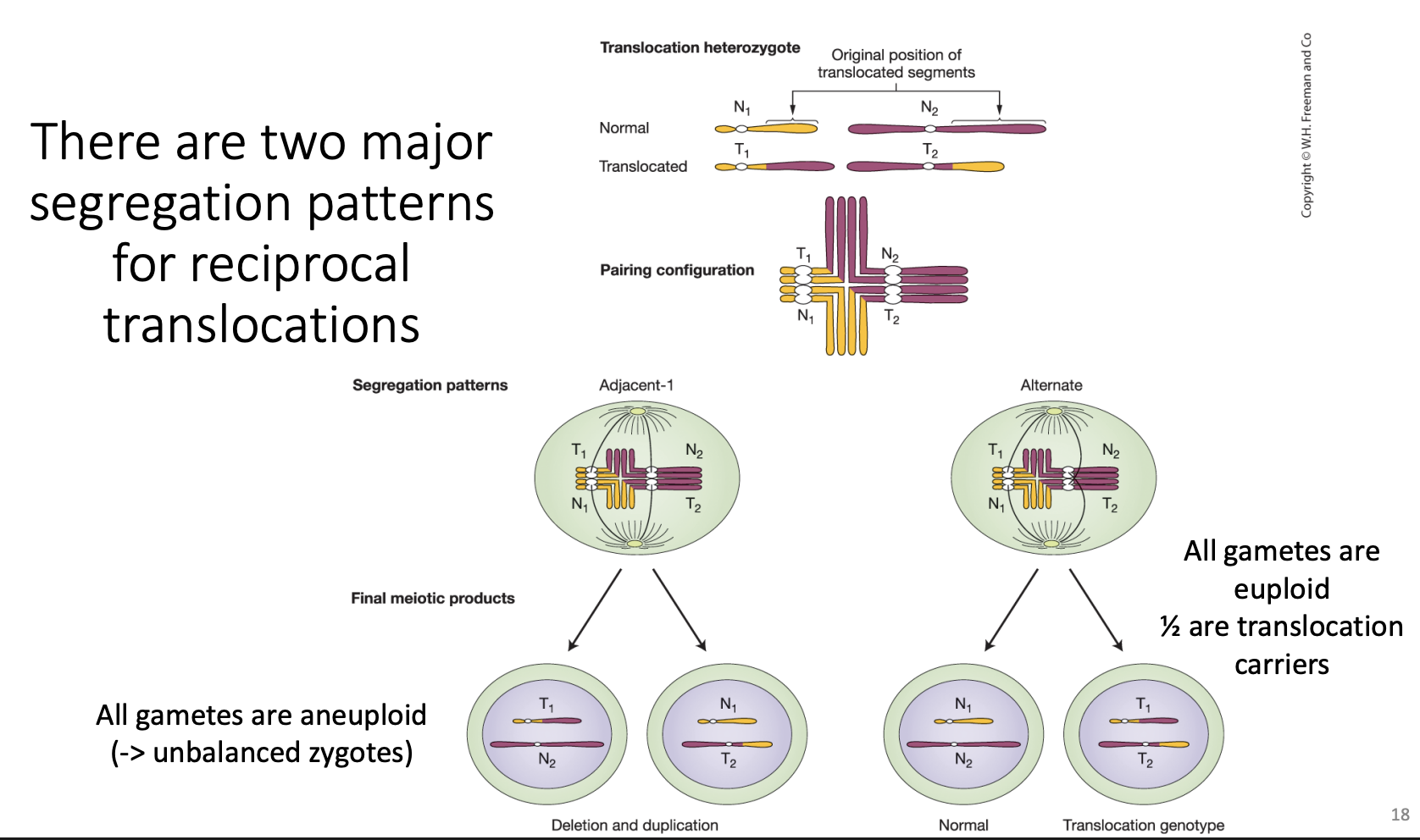
cross-shaped pairing

In prophase I, the four chromosomes (N₁, T₁, N₂, T₂) pair so that homologous regions match up, which creates a cross-shaped quadrivalent. Then it can segregate in different ways:

• Alternate segregation: N₁ and N₂ go to one pole, T₁ and T₂ to the other. Each gamete gets a complete, balanced set. All gametes are euploid: ½ are normal and ½ are translocation carriers.

• Adjacent-1 segregation: neighboring (nonhomologous) centromeres go together (e.g., T₁ with N₂). Every gamete has a duplication of one segment and deletion of another. All gametes are aneuploid, giving unbalanced zygotes that usually die.

So a translocation heterozygote typically has ~50% viable gametes (semisterility) and a carrier is healthy but has reduced fertility and often miscarriages.

Overall goi1Δ::DrugR workflow

Notation: goi1 is “gene of interest 1”. Δ means deleted. :: means “replaced by”. So goi1Δ::DrugR is “goi1 deleted and replaced by a drug resistance gene.”

Diagram: wild-type GOI1 has a pink flanking region on the left and a blue one on the right. The construct has the same pink and blue flanks, but DRG^R (drug resistance gene) sits in the middle instead of GOI1. The matching flanks are the whole point.

Steps:

1. Start with the wild-type gene.

2. Make the deletion construct (order it synthesized and/or PCR it).

3. Transform it into cells (yeast, mouse embryonic stem cells).

4. Select cells that have the DrugR marker by growing them on the drug. Only cells that took up the DNA survive.

5. Verify the genotype, meaning correct integration, usually by PCR. Drug resistance only tells you the marker got in somewhere, not that it went in the right place.

6. Characterize the phenotype in a homozygous organism. For a recessive loss-of-function allele you need both copies gone to see the effect. In yeast (haploid) this is automatic. In mice you breed heterozygotes to get homozygotes.

Drug Resistance Gene:

• Why use it? It lets you select for cells that took up the construct. Transformation is rare, so you need a way to find the few cells that got the DNA.

• Selection or screen? This is a selection: only the cells you want survive, and everything else dies. A screen means everything survives and you look through it to find what you want.

• What if we used a fluorescent protein? That would be a screen. All cells grow, and you pick the glowing ones by eye or by sorting. Same idea (a marker for “has the construct”), different method.

Slide 9: The yeast deletion library

Thousands of strains, each with one gene deleted.

Diagram, top: the construct (top bar) lines up with the yeast chromosome (bottom bar), and the X’s show crossovers. The yeast ORF (orange) runs from ATG to TAA (start to stop), and the whole ORF gets replaced by:

• kanMX4: the drug resistance gene (confers G418/geneticin resistance)

• UPTAG and DNTAG: unique DNA barcodes, one on each side

Diagram, bottom: the final deleted allele, with PCR primers (black arrows, e.g., B-U1, B-U2-comp) that anneal near the barcodes.

Key points:

• Every strain has two unique barcodes, so each strain has a “name tag” in DNA.

• PCR plus sequencing identifies which strain is which. This matters because you can pool all strains together and still tell them apart.

You have ~6000 yeast strains, each missing a different gene. You want to know: which genes does yeast need to grow when food is scarce?

You could test each strain separately (6000 flasks), or you can put them all in one flask and let them compete. Slide 10 is the one-flask version.

Think of it as a race

Imagine 6000 runners in one race, each wearing a unique number (the barcode). Some runners are missing a leg (the deleted gene matters), and some are only missing a hat (the deleted gene doesn’t matter).

• Runners missing a hat keep up.

• Runners missing a leg fall behind and eventually drop out of the pack.

At the end you just count the numbers still in the race, and the runners who disappeared tell you which “body parts” mattered.

Step by step

1. Grow each mutant individually on solid rich media.
Each strain is grown on its own plate with lots of food. Under these easy conditions, the strains grow fine, so every strain starts out healthy. You need this to get enough cells of each strain.

2. Combine them into one flask (YPD = rich liquid medium).
Mix equal amounts of all strains into one flask. Now it’s a mixed population where each strain is roughly equally represented, and each is still identifiable by its barcode.

3. Shift to nutrient-limited conditions (low phosphate or low leucine).
Move the mix to media that is short on one nutrient. Now the strains compete for scarce food.

• A strain missing a gene needed to cope with low phosphate grows slowly.

• A strain missing an unrelated gene grows normally.

4. After several weeks, sequence the barcodes.
Because growth differences are small per generation, you need many generations for them to add up. A strain that grows 5% slower will be a smaller and smaller fraction of the flask over time. After weeks, the slow growers have dwindled or vanished. Then you extract DNA, PCR the barcodes (see the primer explanation), and sequence them to count how many of each there are.

The logic with a toy example

Say you start with 3 strains at equal amounts (33% each):

Strain	Deleted gene	Start	After weeks in low phosphate
A	Gene 1 (unrelated)	33%	50%
B	Gene 2 (helps use phosphate)	33%	1%
C	Gene 3 (unrelated)	33%	49%

Barcode B nearly vanished, so Gene 2 is required for growth in low phosphate. Barcodes A and C stuck around, so those genes aren’t needed under that condition.

Why this is powerful

• One flask tests thousands of genes at once.

• The barcodes let you tell strains apart despite being mixed.

• The same library can be reused for many conditions (low phosphate, low leucine, drugs, heat, and so on).

Things worth knowing for the test

• This is a competition-based screen. The result comes from differences in growth rate over time.

• “Barcode goes away” = gene needed for that condition. It answers “what is this gene needed for?”, which is a reverse genetics question (you started with all the genes known and tested their function).

• Compare to the rich-media (starting) sample. A barcode that’s missing might have been missing at the start for another reason, so you compare the nutrient-limited result to the start or to a control.

• Essential genes aren’t in the knockout pool as viable haploids, so this method tests genes that can be deleted (nonessential in rich media, but possibly needed under special conditions).

deletion strategy

Top diagram: the gene in the genome. Parts to know:

• Promoter region: where transcription starts.

• Start codon (ATG) and stop codon.

• Exons (green) and introns (the lines between them, which get spliced out).

• Splice sites: introns begin with gt and end with ag.

• 3'-UTR with polyA: the end of the mRNA.

• Yellow boxes on the squiggly line are distant regulatory elements (enhancers).

Middle: the deletion construct. Same flanks, but the coding region is replaced by the DrugR marker. Dotted crisscross lines show which sequences pair up for recombination.

Bottom: “Inserting the DRG^R gene requires a double-stranded break.” The chromosome (dot = centromere) has GOI1, and the DRG^R piece with its homologous ends needs the chromosome to be broken to swap in.

Yeast vs mouse

Yeast: when the construct gets in, the cell almost always uses homologous recombination (HR). It sees the matching flanks, lines them up, and swaps the construct in for the gene. Result: >90% correct.

Mouse (and many other eukaryotes): the cell mostly uses NHEJ instead. It doesn’t bother matching the flanks and just glues the DNA into whatever break it finds. Result: <10% correct.

Think of two mail carriers. The yeast carrier reads the address and delivers to the right house. The mouse carrier drops the package at the first open door.

Slides 14-15: the two “wrong” outcomes

In both, the drug resistance gene works, so the cell survives the drug. But the original gene is still intact, so you haven’t knocked anything out.

Slide 14: concatemer

• Many copies of the construct get stuck together end-to-end like a chain, then inserted into the genome somewhere random.

• The native gene is untouched.

Slide 15: single random insertion

• One copy of the construct lands at a random spot in the genome.

• The native gene is untouched.

Correction on the “+” sign

I explained the “+” wrongly before. On the slides it just means “and”: native gene unaltered + construct integrated elsewhere. So the cell has both the normal gene (still working) and the extra marker somewhere else. It does not mean two chromosome copies.

Homology-Dependent Repair (HDR)

• Uses a homologous template: the sister chromatid, the homolog, or supplied donor DNA.

• Mechanism: strand invasion, then double Holliday junction formation (the dashed box).

• A homologous repair template is required (in red on the slide).

• It’s accurate because the cell copies from a template.

NHEJ (Nonhomologous End Joining)

• Just ligates the broken ends together.

• No template required.

• It’s error-prone: ligation often occurs after a few nucleotides are deleted or added. The green block on the chromosome is that small change.

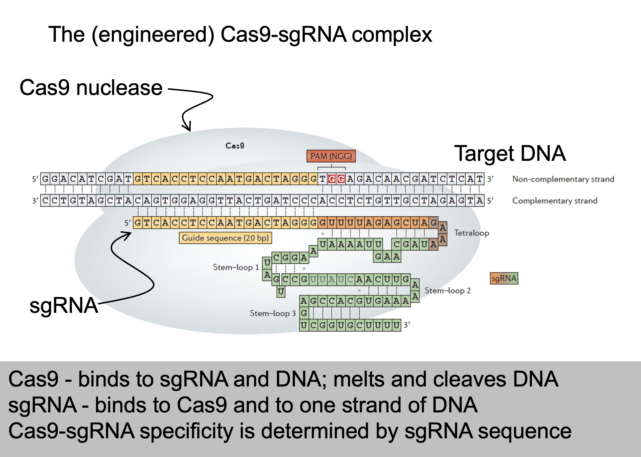
The engineered Cas9-sgRNA complex

• Grey blob = Cas9 nuclease.

• Target DNA (top, two strands) has two labeled strands:

  • Non-complementary strand: has the PAM (NGG), shown in red.

  • Complementary strand: the one the guide RNA base-pairs with.

• sgRNA (the colored RNA under the DNA) has two parts:

  • Guide sequence (20 nt, orange): pairs with the target DNA. This is the part you change to retarget Cas9.

  • Scaffold (green): a tetraloop plus stem-loops 1-3 that bind Cas9. It’s the same for every target.

• Summary box:

  • Cas9 binds sgRNA and DNA, melts and cleaves DNA.

  • sgRNA binds Cas9 and one strand of DNA.

  • Specificity is determined by the sgRNA sequence.
    
    Slide 26: Cleavage site

    The scissors show the cut: both strands are cleaved, a few bases (about 3 bp) upstream of the PAM. The cut leaves ends with a 3'-OH and a 5'-phosphate, the groups ligase needs. The cleavage site is predictable with a high degree of certainty.

Cas9-sgRNA key facts

• Comes from bacterial adaptive immunity. CRISPR = Clustered Regularly Interspaced Short Palindromic Repeats.

• Target must match the sgRNA sequence plus a 3' NGG (PAM).

• sgRNA finds the target by base pairing.

• Cas9 first binds NGG as it scans the DNA, then checks the guide match.

• NGG frequency: N is any base (1), and G and G are each 1 in 4. So 1 × 0.25 × 0.25 = 1/16, about once every 16 bp per strand. Almost any gene has a usable site.

• Cas9 and sgRNA genes are easy to synthesize, so retargeting is cheap.

haploinsufficiency

An essential gene is one the organism needs to survive. If both working copies are gone, the organism (or cell) can’t live. That’s a problem for reverse genetics: you can’t study what a gene does by deleting it if the deletion kills the organism before you can observe anything.

Yeast

Haploid yeast has only one copy of each gene. Delete an essential gene and there’s no backup, so the cell dies. You can’t even grow a strain to study.

Diploid yeast has two copies. If you delete just one (a heterozygous deletion), the cell still has one working copy, so it usually survives. Sometimes it grows slowly, and that is haploinsufficiency: one copy doesn’t make enough protein for normal growth, so you need both copies for full function.

Expressing a protein-coding gene

Flow: DNA gene → (transcription) → mRNA → (translation) → polypeptide → (folding and chemical modifications) → functional protein.

The strands (a favorite exam trick):

• The template (antisense) strand is the one RNA polymerase reads.

• The sense strand is the other DNA strand. Its sequence matches the mRNA, except T becomes U in RNA.

• The mRNA is complementary to the template and identical to the sense strand.

Start and stop: the DNA reads ATG at the start and TAG at the stop. In mRNA these are AUG (codes for Met) and UAG (stop).

Prokaryote point: transcription and translation both happen in the cytoplasm, with no nucleus and no splicing.

Expressing a protein-coding gene (eukaryotes)

Eukaryotes have extra steps:

• The gene has exons (coding) and introns (non-coding, removed).

• The first transcript is a precursor RNA.

• It undergoes splicing (introns out), a 5′ cap (7-mG), a poly-A tail (AAAAA), and sometimes editing.

• The result is the processed (mature) mRNA, which is then translated.

Why it’s here: it shows that eukaryotes have more places to regulate (splicing, capping, and so on). Today is prokaryotes only, where it’s simpler.

What “A is dominant to a” means

Dominance just means: when a cell has both alleles, whose effect do you see?

• If you see A’s effect, A is dominant to a.

• If you see a’s effect, A is recessive to a.

On that slide, A = the working regulatory allele and a = the broken/different version. “A is dominant to a” means “the cell behaves as if the working regulator is doing its job, even though a broken copy is also there.”

(The letters A/a and B/b are generic placeholders. B is the target gene being regulated.)

---

Case 1: A is a protein (trans-acting factor)

The A protein is a diffusible product. Once it’s made, it floats around the cell and reaches every copy of B, wherever it sits.

Trans:  A  b        Cis:  A  B
        a  B              a  b

• Trans arrangement: the A protein reaches B on the other chromosome. B is regulated. ✔

• Cis arrangement: the A protein reaches B on the same chromosome. B is regulated. ✔

Either way you see A’s effect, so A is dominant to a in both cis and trans. The arrangement doesn’t matter. This is called simple dominance.

Lac version: I⁺ (working repressor) vs I⁻ (no repressor). In I⁺ Z⁻ / I⁻ Z⁺ the repressor made by I⁺ diffuses over to the Z⁺ gene and shuts it off, so the cell is inducible (normal). Here I⁺ is dominant to I⁻.

---

Case 2: A is a DNA site (cis-acting element)

A site is just a stretch of DNA. It can’t float anywhere, so it only controls the gene attached to the same DNA molecule.

• Cis arrangement (A B / a b): A sits right next to B, so it regulates B. ✔ You see A’s effect, so A acts dominant.

• Trans arrangement (A b / a B): A sits next to b, on the other chromosome from B. It can’t reach B. B is sitting next to the a site, so B is controlled (or not controlled) the way a dictates. You see a’s effect, so A is recessive.

So with a cis-acting element, dominance depends on where the alleles are (same DNA vs different DNA). That’s why it’s called cis-dominant.

why would a cell turn a gene ON when the substrate shows up?

Break it into pieces

• Substrate = the thing an enzyme breaks down. For lac, the substrate is lactose.

• Gene products = the proteins the genes make. For lac, that’s β-galactosidase (breaks down lactose) and permease (brings lactose into the cell).

• “Needed to use the substrate” = those proteins are the tools for digesting lactose. Without them, lactose is useless to the cell.

So the sentence says: the genes make the tools for using lactose, so the cell should only build the tools when there’s lactose to use them on.

The logic, step by step

Situation	What the cell “thinks”	What happens
No lactose	“Nothing to digest. Making digestive enzymes would waste energy.”	Repressor stays on the operator → genes OFF
Lactose present	“Food is here! I need the tools now.”	Lactose acts as the inducer → repressor falls off → genes ON

An analogy: a restaurant doesn’t fire up the pizza oven until someone orders pizza. The order (substrate) is the signal to start the oven (make the enzymes).

Why this matters for the “inducible” label

This is what makes the system inducible: the substrate itself is the signal that induces (turns on) transcription. And it’s why inducible systems show up in catabolic (breaking-down) pathways. The cell is breaking something down, so the thing being broken down is the trigger.

Contrast with the other type (slide 10, bottom)

For repressible systems (anabolic, building-up pathways), the logic flips:

• The genes make the tools for making a product.

• When the product is plentiful, the cell no longer needs the tools, so the product shuts the genes off.

	Inducible	Repressible
Genes make tools to...	use a substrate	make a product
Signal molecule	the substrate	the product
Signal does	turns genes ON	turns genes OFF
Why	“Food’s here, start digesting”	“Plenty made, stop making more”

One-line takeaway

Catabolic → substrate turns genes ON (use it when it’s there). Anabolic → product turns genes OFF (stop making it when you have enough).

REPRESSIBLE transcription

• Left: the aporepressor is inactive, so RNA polymerase transcribes (default ON).

• The co-repressor (the product) binds the aporepressor.

• Right: this makes an active repressor, which binds the DNA, so no transcription.

• Found in anabolic (biosynthetic) pathways.

• Logic: the product shuts down transcription, because the gene products are needed to make that substance. When enough is made, stop. (The trp operon is the example next lecture.)

INDUCIBLE transcription

• Left: the repressor is bound to the DNA (yellow region). RNA polymerase can’t get in, so no transcription.

• The inducer (the substrate) binds the repressor.

• Right: the repressor becomes an inactive repressor and falls off, so RNA polymerase transcribes.

• Found in catabolic (degradative) pathways.

• Logic: the substrate induces transcription, because the gene products are needed to use the substrate. (“Lactose present → make lactose-digesting enzymes.”)

Lactose utilization by E. coli

E. coli can use lactose for carbon and energy. This needs two proteins:

• Lactose permease (lacY) lets lactose into the cell efficiently.

• β-galactosidase (lacZ) hydrolyzes lactose into galactose + glucose.

Regulation: lactose present → both are made. Lactose absent → neither is made. So lactose induces transcription of lacY and lacZ.

Adaptive value: no wasted resources on enzymes with nothing to digest.

The lac operon model (Jacob and Monod, 1960s)

The map reads: p → o → z → y → a, with transcription going left to right.

• p = promoter

• o = operator, the cis-acting regulatory sequence where the repressor binds

• z, y, a = structural genes (the ORFs):

  • z: β-galactosidase

  • y: lac permease

  • a: lactose transacetylase (the slide says it converts lactose → allolactose and tells you to ignore it)

Definition: the lac operon = the lacZYA transcription unit + its regulatory sequences (promoter and operator).

Note: the slide credits the transacetylase with the lactose → allolactose step. Many textbooks say it’s actually β-galactosidase that makes allolactose, the true inducer. Follow your professor’s slides for the test, but know that the “inducer” is lactose (or its derivative) either way.

Uninducible Mutant Screen

A mutant whose lac operon can’t be turned on, even when lactose is present.

Normally lactose is the signal that switches the operon ON. In an uninducible mutant, that signal does nothing, so the cell never makes β-galactosidase or permease.

Three types of lac cell

Cell type	No lactose	Lactose present
Normal (inducible)	OFF	ON
Constitutive mutant	ON (wrong!)	ON
Uninducible mutant	OFF	OFF (wrong!)

• Constitutive: the switch is stuck ON (always makes enzymes).

• Uninducible: the switch is stuck OFF (never makes enzymes).

Why a cell could be uninducible

Anything that breaks the path from “lactose present” to “enzymes made”:

• A broken lacZ or lacY gene (the enzyme itself is dead)

• A broken promoter (P⁻): RNA polymerase can’t start

• A super-repressor (I^S): the repressor can’t bind lactose, so it never lets go of the operator

(That’s why later slides sort these mutants into types.)

Why the screen on slide 22 works

The key idea: a cell that can’t use lactose can’t live on lactose as its only food.

1. Glycerol plate: glycerol is food the cell can use without lac enzymes, so every colony grows. This is your backup copy.

2. Lactose plate: the only food is lactose. Normal cells switch on the lac operon and grow. Uninducible cells can’t make the enzymes, so they starve and don’t grow.

3. Compare the plates: a spot present on glycerol but missing on lactose is an uninducible (Lac⁻) mutant. You pick it from the glycerol plate, where it’s still alive.

Glycerol plate:  ■ ■ ■ ■ ■ ■   (all grow)
Lactose plate:   ■ ■ _ ■ ■ ■   (gap = Lac⁻ mutant)

Slide 23, constitutive screen (for contrast)

• Here you look for cells that make enzymes when they shouldn’t.

• X-gal turns blue when β-galactosidase cuts it.

• On a glycerol + X-gal plate there’s no lactose, so normal colonies stay white. A blue colony is making β-gal without lactose, so it’s constitutive (Lac^C).

Screen for constitutive mutants (Lac^C)

• Here you look for cells that make enzymes when they shouldn’t.

• X-gal turns blue when β-galactosidase cuts it.

• On a glycerol + X-gal plate there’s no lactose, so normal colonies stay white. A blue colony is making β-gal without lactose, so it’s constitutive (Lac^C)

1. Patch colonies onto glycerol + X-gal. There’s no lactose, so a normal colony stays white/cream, because the operon is OFF.

2. A colony that turns blue on glycerol is making β-gal without lactose, so it is constitutive (Lac^C).

3. On lactose + X-gal, all colonies turn blue (everyone can induce).

Logic: blue on a non-inducing plate means the operon is stuck ON. Recover it for study.

Result: hundreds of Lac^C mutants.

Making a merodiploid

Four stages (top to bottom):

1. F⁺ cell: F is “episomal” (separate from the chromosome). The chromosome carries lac.

2. Hfr cell (“high frequency recombination”): the F factor integrates into the chromosome.

3. F′ cell: F excises (pops out) but this time takes a piece of the chromosome with it, including lac. It’s now called F′ (F-prime).

4. F′ is transferred by conjugation into an F⁻ cell. The result is F′ lac / lac = a merodiploid (partial diploid), with two copies of lac: one on the chromosome, one on F′.

Merodiploid = a bacterial partial diploid you can use for complementation and cis/trans tests.

Conjugative F plasmids

• F plasmid: a circular piece of DNA separate from the chromosome.

• A donor (F⁺) cell connects to a recipient (F⁻) cell and transfers a copy of F. Both cells end up F⁺.

• This is conjugation, the transfer of DNA between cells.

Regulatory constitutive mutants, O^c

• Mapped to one location: lacO, the operator. “O” is for operator, a cis-acting element.

• O^c (operator-constitutive) mutations change the operator so the repressor can’t bind it.

Merodiploids:

• O^c Z⁺ / O⁺ Z⁻ (cis): constitutive. O^c is on the same DNA as Z⁺, the repressor can’t bind there, and Z⁺ is always transcribed. The O⁺ on the other chromosome doesn’t help, because it only controls the Z⁻ next to it.

• O^c Z⁻ / O⁺ Z⁺ (trans): inducible. O^c only affects the dead Z⁻ on its own chromosome. The Z⁺ has a normal operator, so regulation is normal.

Conclusion: O^c is dominant in cis but recessive in trans. This is the classic cis-acting element result.

Regulatory uninducible mutants, P⁻

• A single complementation group, mapped very close to lacZ: lacP. “P” is for promoter, a cis-acting element.

• P⁻ is a loss-of-function mutation in the promoter, so RNA polymerase can’t transcribe: uninducible.

Merodiploids:

• P⁻ Z⁺ / P⁺ Z⁻ (cis): uninducible. Z⁺ has the broken promoter. The other chromosome has a good promoter but a dead Z gene.

• P⁻ Z⁻ / P⁺ Z⁺ (trans): inducible. Z⁺ has a good promoter.

Conclusion: P⁻ is dominant in cis but recessive in trans, the same pattern as O^c.

Careful: O^c and P⁻ have the same cis/trans dominance pattern but opposite phenotypes (constitutive vs uninducible).

lac mutant chart

Slide	Content	Key result
2	Lac operon model; mutants were constitutive or uninducible	Led to the trans/cis hypothesis
3	Merodiploids: F′lac^m1 / lac^m2	How complementation works in haploid bacteria
4	lacZ⁻ / lacY⁻ (structural)	Recessive; two complementation groups
5	lacI⁻ (constitutive)	Recessive in cis AND trans
6	O^c (constitutive)	Dominant in cis, recessive in trans
7	P⁻ (uninducible)	Dominant in cis, recessive in trans
8	lacI^S (uninducible)	Dominant in cis AND trans
9	Recap: cis-acting elements	Only affect the gene on the same DNA
10	Recap: trans-acting factors	Dominant allele acts on all copies

New details worth noting:

• Slide 8 note: I^S is a gain of function for repression (it represses too well) but a loss of function for lactose binding. That’s why it can be both.

• Slide 10: “these act on all alleles” means a diffusible protein reaches every copy of the target gene.

Strong vs weak promoters

Reminder: the −35 consensus is TTGACA (initial recognition by RNA polymerase). The −10 consensus is TATAAT (DNA melting starts).

• Slide 13: the trp promoter has a perfect match to the consensus at the −35 initial recognition site. RNA polymerase recognizes it well.

• Slide 14, strong promoters: the red arrows and boxes mark trp and leu, whose −35 regions match TTGACA exactly.

• Slide 15, weak promoters: the blue arrows mark lacI and bio. The blue circles mark bases that don’t match the consensus.

Rule:

Closer to consensus → stronger promoter. More mismatches → weaker promoter.

A strong promoter doesn’t need help, so it’s fine for trp to be controlled by a repressor alone. A weak promoter needs an activator, which sets up slide 16.

How CRP works

The activator: CRP (cAMP Receptor Protein) complexed with cAMP.

• It binds the cAMP Response Element (cre), a cis-acting element next to the lac promoter.

• Bound, it helps RNA polymerase bind and transcribe.

The two pictures:

• − glucose, + lactose (top): cAMP is available → cAMP binds CRP → the cAMP-CRP complex sits at cre → RNA Pol transcribes z, y, a (red arrow).

• + glucose, + lactose (bottom): glucose blocks cAMP synthesis, so CRP has no cAMP (the red X over cAMP), can’t bind, and the promoter isn’t activated.

Summary: glucose present → no cAMP → no active CRP → lac operon can’t be turned up.

Combinatorial control

The lac operon is controlled by two inputs at once:

• Negative: the LacI repressor (responds to lactose).

• Positive: cAMP-CRP (responds to glucose).

Glucose	Lactose	Repressor	cAMP-CRP	lac mRNA?
−	+	Off the operator (lactose bound it)	Bound, activates	YES
−	−	On operator	Bound	NO (repressor blocks)
+	−	On operator	Absent	NO
+	+	Off the operator	Absent	NO (no activator, weak promoter)

Takeaway: the operon is ON only when lactose is present AND glucose is absent. It works like an AND gate:

• No lactose → no point making the enzymes → repressor blocks.

• Glucose present → better food available → no activator.

Genetic evidence for the glucose mechanism

Background: cAMP is made by adenylate cyclase (gene cya), which is inhibited by glucose. CRP is encoded by crp.

The table (both conditions have lactose):

Genotype	+ Lac, + Glucose	+ Lac, − Glucose
cya⁺ crp⁺ (normal)	cAMP low → No transcription	cAMP high → Yes
cya⁻ crp⁺	cAMP low → No	cAMP low → No
cya⁺ crp⁻	cAMP low → No	cAMP high → No

How to read it:

• Normal: glucose gone → cAMP rises → transcription.

• cya⁻: can’t make cAMP, so even without glucose cAMP stays low → no transcription.

• crp⁻: cAMP is made (high) but there’s no CRP to receive it → no transcription.

Conclusion: you need both cAMP and working CRP. Both mutants are uninducible even though lactose is present.

Gal transcriptional Activators/repressors

Slide 24: GAL genes are NOT an operon (NEW)

Eukaryotes generally don’t make polycistronic mRNAs (the contrast from Lecture 21 slide 13). So how are the three genes coordinated?

The picture: GAL7, GAL10, GAL1 sit near each other, but:

• Each has its own promoter and its own transcription (the “Txn” arrows; GAL7 and GAL10 go left, GAL1 goes right).

• Each promoter is controlled by similar cis-acting elements called Upstream Activation Sequences (UAS), the dark blue bars.

• The UAS elements are bound by one shared trans-acting factor: GAL4p (the red circles).

Answer: coordination comes from one shared activator controlling several separate genes, not from one shared mRNA.

---

Slide 25: Gal4p is a transcriptional activator (NEW)

The monomer has two domains:

• A zinc-finger DNA-binding domain (red ball): grabs the UAS.

• A transcription activation domain (green): recruits RNA polymerase.

It works as a homodimer (two copies), like many transcription factors.

Function: when Gal4p is bound to the UAS, it recruits the RNA polymerase complex (RP) to the promoter → transcription of GAL1, GAL7, GAL10. The bottom picture shows dimers on every UAS with polymerase (blue) at all three promoters.

---

Slide 26: Gal80p blocks Gal4p when there’s no galactose (NEW)

• Gal80p (purple chevrons) binds the Gal4p activation domain.

• This blocks polymerase recruitment. Gal4p is still sitting on the UAS, but it’s silenced.

• Bottom picture, “when no galactose present”: the dashed arrows show little or no transcription.

So Gal80p is a co-repressor of Gal4p. It doesn’t bind DNA itself. It sits on the activator.

---

Slide 27: Gal3p senses galactose (NEW)

Key (top left): galactose = star, Gal3p = orange square, Gal3p/galactose complex = star on the square.

Mechanism: with galactose present:

1. Galactose binds Gal3p.

2. The Gal3p/galactose complex binds Gal80p, pulling it off Gal4p’s activation domain.

3. Gal4p is free to recruit RNA polymerase → transcription ON.

The bottom picture: lots of orange squares with stars carrying the purple Gal80p away, and polymerase at all three genes.

---

Slide 28: Glucose control, MIG1p (NEW)

Mechanism: with glucose present, the repressor MIG1p blocks transcription of the GAL4 gene itself.

• No Gal4p is made (the red X over Gal4p).

• So GAL1, 7, 10 can’t be expressed, even if galactose is present.

• Bottom picture: no activators, RNA polymerase (blue) floating unused.

This is the glucose-over-galactose rule, like CRP in E. coli, but done in a different way.

Predicting mutants and epistasis

The note says all phenotypes are without glucose, so MIG1p isn’t repressing.

Mutant	Phenotype	Why
gal3⁻	Uninducible	Without Gal3p, Gal80p is never removed, so Gal4p stays blocked even with galactose
gal80⁻	Constitutive	Without Gal80p nothing blocks Gal4p, so genes are on even without galactose
gal3⁻ gal80⁻	Constitutive	With no Gal80p, Gal3p has nothing to act on

Epistasis in plain words: in a double mutant, the phenotype matches one of the single mutants. The gene whose phenotype wins is epistatic. Here the double mutant looks like gal80⁻, so GAL80 is epistatic to GAL3.

Rule from the slide:

In a regulatory pathway, the epistatic gene is the downstream gene.

Gal80p is downstream of Gal3p (Gal3p acts on Gal80p), so Gal80p wins.

The Shh limb enhancer

Main point: the limb-specific enhancer for the Shh gene is about 1 megabase away from Shh, inside an intron of a different gene (LMBR1).

Slide 14 pictures:

• A: map showing the limb enhancer (red) in the LMBR1 region, and the Shh gene (blue) a megabase away.

• B: two mice. The wild-type mouse is normal. The mouse with the limb enhancer deleted has severely truncated limbs.

• C-E: human hands from patients with point mutations in the enhancer. They have extra digits (preaxial polydactyly). Panel E shows the DNA sequences.

Slide bullets:

• Point mutations in humans disrupt the pattern of Shh expression during development.

• Deletion in mice eliminates expression.

Key idea: the Shh gene itself is normal. The mutations are in a non-coding enhancer far away, and they still cause a phenotype. This is how cis-acting elements are studied.

Slide 15: the reporter experiment

• The enhancer DNA is attached to a lacZ reporter gene (red box = enhancer, blue box = lacZ) and put into a mouse embryo.

• Wherever the enhancer is active, β-galactosidase is made. X-gal turns it blue (the same trick as the lac lecture).

• The mouse embryo picture shows blue spots in the limb buds, so the enhancer drives expression in limbs.

---

How do distant enhancers work? Looping and insulators

• Observation (top): one gene’s mRNA is expressed in the brain and limb. The “?” marks are unknown locations of the enhancers.

• Brain panel: brain-expressed transcription factors (TFs) bind the brain enhancer (blue). With a co-activator (starburst), the DNA loops so the enhancer touches the promoter with RNA Pol II (“P”). This gives brain mRNA. The limb enhancer (green) stays inactive.

• Limb panel: limb-expressed TFs bind the limb enhancer (green), which loops to the promoter, giving limb mRNA.

• Red STOP signs = insulators.

Key points:

• An enhancer is only active in tissues that have the right set of TFs. Different tissues use different enhancers for the same gene.

• Enhancers act by looping: the DNA bends so a distant enhancer physically touches the promoter.

Insulator elements: block enhancer-promoter interactions. They restrict an enhancer to a defined chromatin domain so it doesn’t turn on other nearby genes.

---

The methylation cycle

The picture shows CpG sites on both strands. CpG is palindromic: the C-G on one strand pairs with a C-G on the other, so both strands carry a methylatable C (“Me” above and below).

Slide	Process	What happens
25 (1)	De novo methylation by DNMT3A/3B	Adds methyl groups to an unmethylated CpG site. Can establish a repressed state in response to the developmental program or environment.
26 (2)	DNA replication, then passive demethylation	After replication, each daughter DNA has the old strand methylated and the new strand not. This is a hemimethylated CpG site. If nothing fixes it, the next replication produces unmethylated DNA. Methylation is lost “passively” over cell divisions.
27 (3)	Maintenance methylation by DNMT1	DNMT1 sees the hemimethylated site and methylates the new strand, restoring full methylation. It keeps the repressed state through cell divisions and gives cellular “memory” of past decisions.
28 (4)	Active demethylation by demethylases	Enzymes remove methyl groups directly. The repressed state is reversible, as in the germline and early embryo, or in response to environmental factors.

Memory trick:

• DNMT3A/3B = new (de novo)

• DNMT1 = copies the pattern after replication (maintenance)

• Demethylases = erase (active)

• No maintenance = methylation fades (passive)

---

Slide 29: Methylated CpG islands

• 300-3000 nucleotides long, with high CpG content.

• Methylation silences gene expression.

• Often found in transposons (methylation suppresses hopping).

• 60-70% of CpGs are methylated in human somatic cells.

Slide 34: the UCSC Human Genome Browser view of LMBR1.

• Shows LMBR1 exons (black boxes) and alternatively spliced LMBR1 mRNAs (many rows).

• The conservation track (“100 vertebrates”) has peaks where sequence is conserved.

• Blue arrows: conserved peaks that line up with known exons.

• Red arrows with “?”: conserved peaks that don’t match a known exon. What are they?

• One exon is boxed for zooming.

Slide 35: zoom in on one exon.

• The aligned amino acids are shown across many vertebrate species and are nearly identical, so the protein sequence is conserved.

• 3-nt periodicity: the conservation graph shows dips at every third position, the 3rd positions of codons, where changes are often synonymous and conservative (they don’t change the amino acid).

• Splice sites are conserved:

  • 5′ splice site: 5′-GURAGU-3′

  • 3′ splice site: 5′-YnYAG-3′ (a stretch of pyrimidines then AG)

• In the flanking intron, changes are non-frame-preserving (no protein to protect).

• Label: “Conserved for protein-coding function (Exon).”

Checklist for an exon: protein-like conservation, 3-nucleotide periodicity, conserved splice sites, and a flanking region that changes freely.

---

Slides 36-37: A conserved sequence that is NOT an exon

Slide 36: the red “?” arrow points to a conserved peak in LMBR1 that isn’t an exon.

Slide 37: zoom in.

• Next to the Shh label, the alignment is strongly conserved across species (zebrafish to human), but:

  • No exon detected by RNA sequencing

  • No periodicity (no 3-nt pattern)

  • Not frame-preserving

  • “Not likely to be conserved for protein-coding function”

Conclusion: something non-coding is being conserved. “An Enhancer? Remember Sonic hedgehog (shh) from the previous lecture!”

Finding an exon of LMBR1 in the genome browser

• Shows LMBR1 exons (black boxes) and alternatively spliced LMBR1 mRNAs (many rows).

• The conservation track (“100 vertebrates”) has peaks where sequence is conserved.

• Blue arrows: conserved peaks that line up with known exons.

• Red arrows with “?”: conserved peaks that don’t match a known exon. What are they?

• One exon is boxed for zooming.

Slide 35: zoom in on one exon.

• The aligned amino acids are shown across many vertebrate species and are nearly identical, so the protein sequence is conserved.

• 3-nt periodicity: the conservation graph shows dips at every third position, the 3rd positions of codons, where changes are often synonymous and conservative (they don’t change the amino acid).

• Splice sites are conserved:

  • 5′ splice site: 5′-GURAGU-3′

  • 3′ splice site: 5′-YnYAG-3′ (a stretch of pyrimidines then AG)

• In the flanking intron, changes are non-frame-preserving (no protein to protect).

• Label: “Conserved for protein-coding function (Exon).”

Checklist for an exon: protein-like conservation, 3-nucleotide periodicity, conserved splice sites, and a flanking region that changes freely.

---

Slides 36-37: A conserved sequence that is NOT an exon

Slide 36: the red “?” arrow points to a conserved peak in LMBR1 that isn’t an exon.

Slide 37: zoom in.

• Next to the Shh label, the alignment is strongly conserved across species (zebrafish to human), but:

  • No exon detected by RNA sequencing

  • No periodicity (no 3-nt pattern)

  • Not frame-preserving

  • “Not likely to be conserved for protein-coding function”

Conclusion: something non-coding is being conserved. “An Enhancer? Remember Sonic hedgehog (shh) from the previous lecture!”

---

Slide 38: Confirmation

That conserved sequence is the Sonic hedgehog enhancer inside the LMBR1 gene!

This slide repeats Lecture 23 slides 14-15: the limb enhancer is ~1 Mb from Shh inside LMBR1, point mutations in humans cause extra digits, deleting it in mice truncates limbs, and a lacZ reporter + X-gal gives blue limb buds in the embryo.

Lesson: conservation analysis predicted a functional non-coding element, and the reporter experiment confirmed it.

How to tell “conserved exon” from “conserved non-coding element”:

Feature	Exon	Non-coding (e.g. enhancer)
Found by RNA-seq	Yes	No
3-nt periodicity	Yes	No
Frame-preserving	Yes	No
Splice sites	Yes	No
Conserved?	Yes	Yes

How mRNA-seq works

1. Extract RNA from cells, tissue, or whole organism with phenol/chloroform. The image shows mRNAs with a 5′ end, an exon (purple), and a poly-A tail (AAA) at the 3′ end.

2. Enrich mRNA using oligo-dT (a string of Ts) attached to magnetic beads. The Ts base-pair with the poly-A tails, and the magnet pulls the mRNAs out. This removes the very abundant rRNA and tRNA, which have no poly-A tails. (The cartoon man with a magnet is just a joke on “magnetic beads.”)

3. Fragment the mRNA chemically (heat + Mg²⁺ at high pH) into ~300 bp pieces. This is because sequencers read short fragments.

Slide 9:
4. Reverse-transcribe the RNA fragments into cDNA with reverse transcriptase. RNA can’t be PCR’d or sequenced directly in this workflow, so it’s converted to DNA. The diagram (Hrdlikova et al., 2016) shows:

• A random-hexamer primer (NNNNNN) anneals to the fragment and RT makes the first cDNA strand.

• RT adds a few extra C’s at the 3′ end (3′ CCC), and a template-switching oligo with GGG pairs with them. RT “switches” and copies the oligo, adding an adapter sequence to the other end of the cDNA.

• Second strand synthesis makes double-stranded DNA.

• (You probably don’t need the template-switching details. Just know RT makes cDNA and adapters get added.)

5. PCR adds sequencing primer sites and a barcode that identifies the sample. The result is a sequencing-ready library. The barcode (the “xxx”) lets you pool multiple samples in one run and sort the reads afterward by barcode.

---

Slide 10 – Sequencing and mapping

6. cDNA sequencing (e.g., Illumina) produces reads, short sequences of the fragments.

7. Map the reads to the genome. The box shows an RNA-seq read ATGCAGACTGCAGACGTCAG matching the genome sequence perfectly (the vertical bars show matches).

   • The diagram shows many blue reads stacked over a green box = exon, and fewer stacked over another green box. Reads only land where RNA was made, so where reads pile up, there’s an exon (“so there’s an exon here... and here”).

   • Number of reads over a gene reflects how much of that mRNA was present.

   • (Extra context, not on slide: reads span exon-exon junctions and don’t cover introns, since introns are spliced out of mature mRNA. That’s how RNA-seq reveals gene structure.)