Chapter 2: Limits and Continuity

A. Definitions and Example

• The number L is the limit of the function f(x) as x approaches c if, as the values of x get arbitrarily close (but not equal) to c, the values of f(x) approach (or equal) L.

  We write: limx→cf(x)=L

• In order for limx→cf(x) to exist, the values of f must tend to the same number L as x approaches c from either the left or the right.

We write limx→c−f(x) or the left-hand limit of f at c (as x approaches c through values less than c).

We write limx→c+f(x) for the right-hand limit of f at c (as x approaches c through values greater than c).

\
Example:

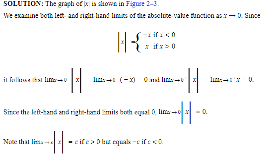
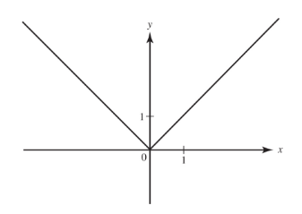
Prove that limx→0|x|=0.

SOLUTION:

Definition

• The function f(x) is said to become infinite (positively or negatively) as x approaches c if f(x) can be made arbitrarily large (positively or negatively) by taking x sufficiently close to c.

We write limx→cf**(x)=+∞ (or limx→cf****(x)=−∞)**

Since, for the limit to exist, it must be a finite number, neither of the preceding limits exists.

• This definition can be extended to include x approaching c from the left or from the right. The following examples illustrate these definitions.

\
Example:

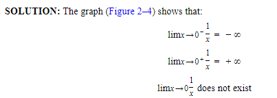
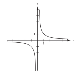
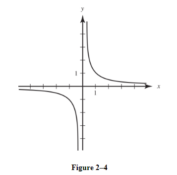
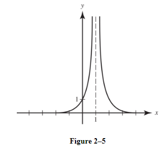
Describe the behavior of f(x)=1/x near x = 0 using limits.

SOLUTION:

\

Definition

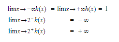
• We write:

limx→∞f(x)=L(or limx→−∞f(x)=L)

if the difference between f(x) and L can be made arbitrarily small by making x sufficiently large positively (or negatively).

Example:

SOLUTION:

B. Asymptotes

• The line y = b is a horizontal asymptote of the graph of y = f(x) if limx→∞f(x)=borlimx→−∞f(x)=b.

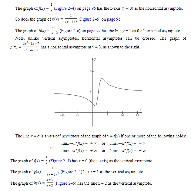
Note, unlike vertical asymptotes, horizontal asymptotes can be crossed.

Example:

\
SOLUTION:

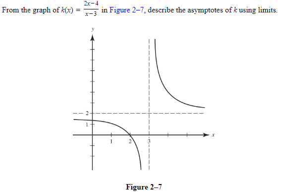
We see that y = 2 is a horizontal asymptote, since

limx→+∞k(x)=limx→−∞k(x)=2

Also, x = 3 is a vertical asymptote; the graph shows that

limx→3−k(x)=−∞ and limx→3+k(x)=+∞

\
\

C. Theorems of Limits

If B, D, E, c, and k are real numbers and if the limits of functions f and g exist at x = c such that limx→cf(x)=B and limx→cg(x)=D then:

1. The Constant Rule: limx→ck=k

2. The Constant Multiple Rule: limx→ck⋅f(x)=k⋅limx→cf(x)=k⋅B

3. The Sum Rule: limx→c(f(x)+g(x))=limx→cf(x)+limx→cg(x)=B+D

4. The Difference Rule: limx→c(f(x)−g(x))=limx→cf(x)−limx→cg(x)=B−D

5. The Product Rule: limx→c(f(x)⋅g(x))=limx→cf(x)⋅limx→cg(x)=B⋅D

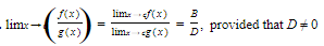
6. The Quotient Rule:

   

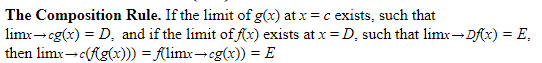
7. The Composition Rule:

   

8. The Squeeze or Sandwich Theorem:

   

   

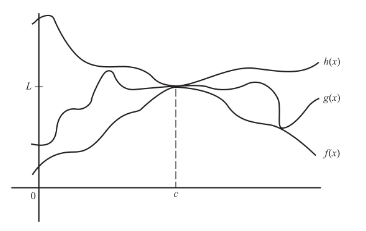
Squeezing function g between functions f and h forces g to have the same limit L at x = c as do f and g.

\
Example:

\n

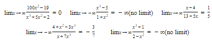
D. Limit of a Qoutient of Polynomials

To find

where P(x) and Q(x) are polynomials in x, we can divide both numerator and denominator by the highest power of x that occurs and use the fact that

Example:

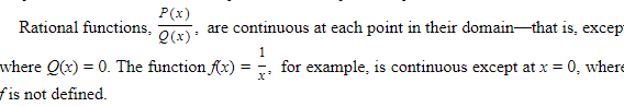
The Rational Function Theorem

This theorem holds also when we replace “x→∞” by “x→−∞.”

Note also that:

\
2.

\
3.

\
\
Example:

\

E. Other Basic Limits

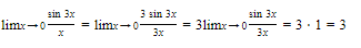
E1. The basic trigonometric limit is:

\
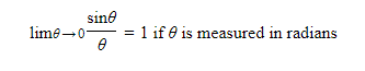
Example:

Solution:

E2. The number e can be defined as follows:

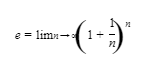
The value of e can be approximated on a graphing calculator to a large number of decimal places by evaluating

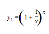
for large values of x.

\

F. Continuity

• If a function is continuous over an interval, we can draw its graph without lifting pencil from paper. The graph has no holes, breaks, or jumps on the interval.
• Conceptually, if f(x) is continuous at a point x = c, then the closer x is to c, the closer f(x) gets to f(c). This is made precise by the following definition:

Definition

The function y = f(x) is continuous at x = c if

1. f(c) exists (that is, c is in the domain of f)
2. limx→cf(x) exists
3. limx→cf(x)=f(c)

• A function is continuous over the closed interval [a,b] if it is continuous at each x such that a ⩽ x ⩽ b.
• A function that is not continuous at x = c is said to be discontinuous at that point. We then call x = c a point of discontinuity.

\

Continuous Functions

• Polynomials are continuous everywhere—namely, at every real number.
• 
• The absolute-value function f(x) = |x|is continuous everywhere.
• The trigonometric, inverse trigonometric, exponential, and logarithmic functions are continuous at each point in their domains.
• Functions of the type n√x (where n is a positive integer ⩾ 2) are continuous at each x for which n√x is defined.
• The greatest-integer function f(x) = [x] is discontinuous at each integer, since it does not have a limit at any integer.

\

Kinds of Discontinuity

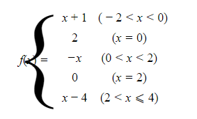
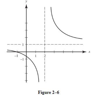
The graph of f is shown at the right.

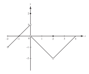
We observe that f is not continuous at x = −2, x = 0, or x = 2.

At x = −2, f is not defined.

At x = 0, f is defined; in fact, f(0) = 2.

• However, since limx→0−f(x)=1 and limx→0+f(x)=0, limx→0f(x) does not exist.
• Where the left- and right-hand limits exist, but are different, the function has a jump discontinuity.
• The greatest-integer function, y = [x], has a jump discontinuity at every integer.

At x = 2, f is defined; in fact, f(2) = 0. Also, limx→2f(x)=−2; the limit exists.

• However, limx→2f(x)≠f(2).
• This discontinuity is called removable.
• If we were to redefine the function at x = 2 to be f(2) = −2, the new function would no longer have a discontinuity there.
• We cannot, however, “remove” a jump discontinuity by any redefinition whatsoever.

Whenever the graph of a function f(x) has the line x = a as a vertical asymptote, then f(x) becomes positively or negatively infinite as x → a+ or as x → a−.

• The function is then said to have an infinite discontinuity.

\
Example:

SOLUTION:

This function is continuous except where the denominator equals 0 (where g has an infinite discontinuity). It is not continuous at x = 3, but is continuous at x = 0.