WM273_Lecture_1_-_Process_Control
Page 3: Control Overview
Control: The process of altering system performance
Purpose: Mass production of consistent products from continuous processes
Reason: Systems do not always behave as desired
Aims:
Regulation: Maintain output variable constant despite disturbances
Tracking: Follow a variable setting
Sequencing: Ensure events occur in a specific sequence
Page 4: Importance of Process Control
Description: Refining, combining, handling, and otherwise manipulating fluids to profitably produce end products can be a precise, demanding, and potentially hazardous process.
Small changes can significantly impact results
Factors to control: variation in proportions, temperature, flow, turbulence, etc- in order to make the desired end product with a minimum of raw materials and energy
Process control technology: Runs operations within limits to maximize profitability, ensure quality, and safety
Page 5: Basic Objectives of Process Control
Objective: Regulate the value of a quantity to maintain a desired value
Activities: Ensure processes are predictable, stable, and consistently at target performance levels
Evolution: Early controls involved human operators; now machines and electronics prevail
Page 6: Process Control Systems
Example: Regulating the level of liquid (Q) in a tank to height (H)
Input flow is unregulated
Liquid flow rate per unit height is illustrated (K), where K is a liquid flow rate per unit of height (h)
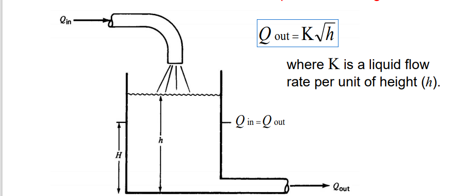
Equations:
Q_out = K * sqrt (h)
Q_in = Q_out
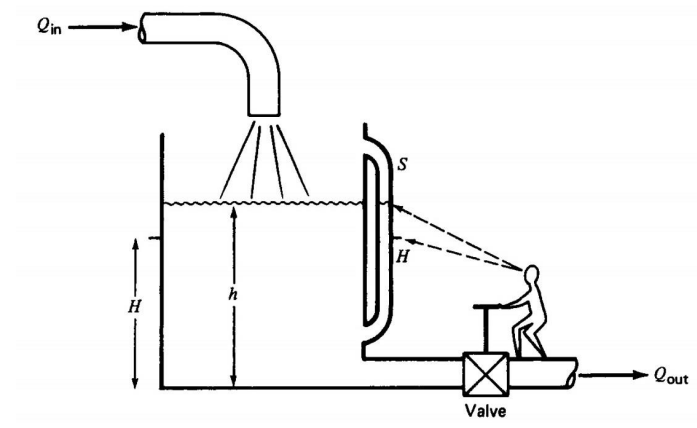
Page 7: Human Regulation in Control Systems
Description: A human compares actual fluid level (h) to objective (H) via a sight tube (S)
Adjustment of output valve as needed
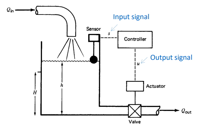
Page 8: Automatic Control Systems
Components of an automatic level-control system:
Sensor: Measures fluid level
Actuator: Adjusts the valve
Controller: Coordinates sensor and actuator
Page 9: Control Variables in Process Control
Variables that can be controlled:
Pressure
Flow rate
Level
Temperature
Density
pH
Liquid interface
Mass
Conductivity
Page 10: Control Variables Management
Elements for regulating variables:
Sensors, transducers, transmitters for information
Manipulative elements (motors, pumps, etc.)
Control elements
Interface elements
Setpoint: Desired value of a variable to maintain, which can be min, max, or within a range around the setpoint
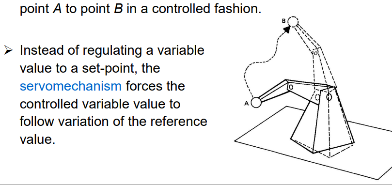
Page 11: Servomechanisms
These control systems have slightly different objectives from process control.
Function: Move a robot arm or similar systems from point A to point B (in a controlled fashion)
Objective differs from basic process control - follows variations of a reference value
Page 12: Discrete-State Control Systems
Controls a sequence of events (flow rate, speed, temperature) rather than the regulation or variation of individual variables.
Events are in a discrete state (ON/OFF)
Can be automatic, often using Programmable Logic Controllers (PLCs)
Some sequence phases can be more accurately controlled
Control Systems and Their Evaluation
Page 14: Open Loop Control
Definition: Inputs are not influenced by output
Control is based on pre-calculations. Apply some input, either fully energizing the actuator(s), or partially energising, based on some off-line pre-calculations.
Disadvantages: Changes in controlled object/environment lead to output deviation
Examples: Electric heater without thermostat, timed sprinklers, many electric motors (hand-held tools, kitchen appliances, some conveyer belts, etc)
Page 15: Open Loop and Closed Loop Basics
Description of disturbance influence on inputs and outputs in control processes
Various components involved in both systems: Inputs, Process/controller, Outputs
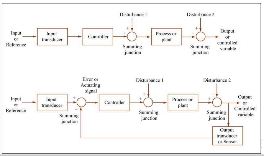
Page 16: Closed Loop Control
Definition: Controlling action IS influenced by the output!
Comparison between requested output and measured output
Process of error reduction (amplification, integration, etc.). The discrepancy (error) is processed (amplified, integrated, etc) in order to generate the best input to the actuator that controls the energy input to the process.
Closed-loop examples: Electric heater with thermostat, cruise control, grass sprinkler with rain & moisture sensors, grass sprinkler with rain & moisture sensors
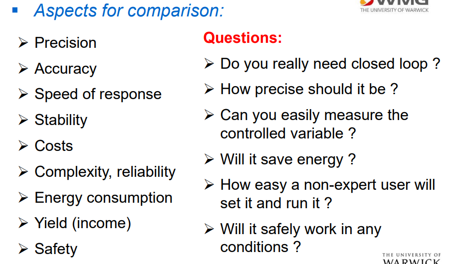
Page 17: Comparison: Open Loop vs Closed Loop
Aspects for comparison: Precision, Accuracy, Speed, Stability, Costs, Complexity, Energy Consumption, Safety
Questions posed for evaluation of control types
Page 18: Control System Evaluation Objectives
Objective: Evaluation based on error size and variation over time
Practical objectives: Stability and the system should provide the best possible steady-state regulation, and transient regulation
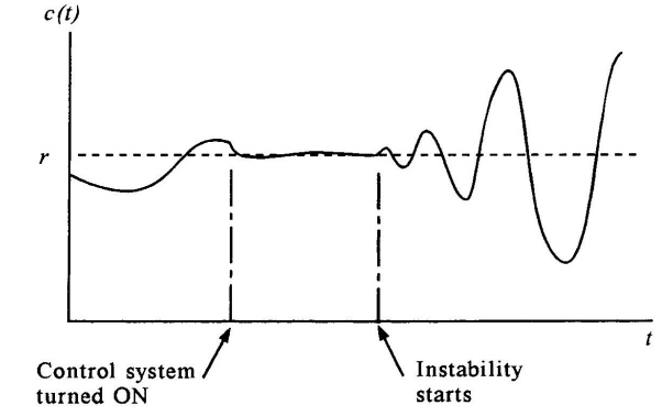
Page 19: Stability in Control Systems
Requirement: Control system must be designed and adjusted for stability
However, as a control system is adjusted to give a better control and a faster response, the likelihood of instability also increases
Page 20: Steady-State and Transient Regulation
Steady State Regulation - Best possible steady-state regulation means minimizing the steady-state error (e)
The transient regulation specifies how the control system reacts to a sudden change or large variation of some process variable in order to reduce such effects on the control system. This is called the control system transient response
Evaluation Criteria - The term tuning is used to indicate how a process-control loop is adjusted to provide the best control
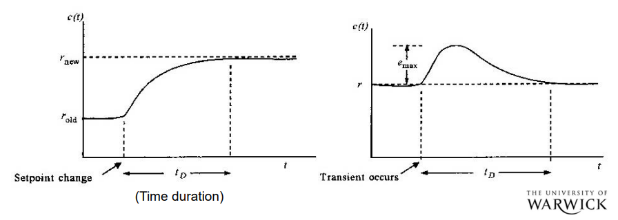
Page 21: Damped Response in Control Systems
One of the performance measures is how the system responds to changes of setpoint or to a transient disturbance
Damped (Aperiodic) Response
For this type of response, measures of quality are the time duration and maximum error. The error (e) is of only one polarity (i.e., it never oscillates about the setpoint (r))
Page 22: Cyclic Response
The output variable exhibits oscillations about the reference value (r), (setpoint).
Parameters of interest: Time duration and maximum error (e)
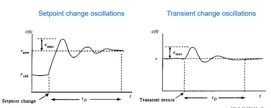
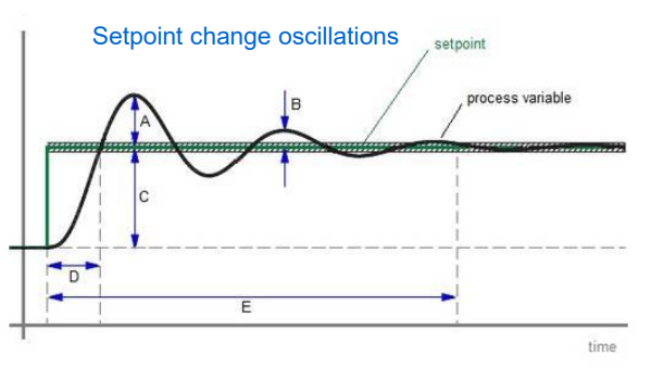
Page 23: Setpoint Change Cyclic Response
Response features defined for step input changes:
A: Overshoot
B: Second overshoot
C: Step input change
D: Rise time
E: Settling time
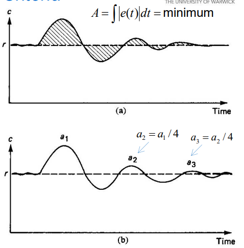
Page 24: Simple Cyclic Tuning Criteria
Minimum Area: Adjust tuning until the shaded area under the error-time curve (net area, A) is minimal (a)
Quarter Amplitude: The amplitude of each peak of the cyclic response is quarter or less of the preceding peak, (b)
Analog and Digital Processing
Page 26: Analog vs Digital Data
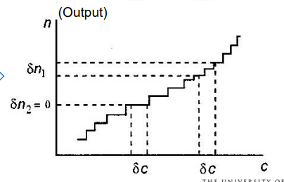
Analog Data: Continuous variation between variable representation and actual value. This type of data means that there is a smooth and continuous variation between representation of a variable value b and the value itself c
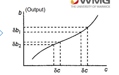
Digital Data: Representation in binary digits (0 or 1). As a result, the variable c is represented by a digital quantity n
Page 27: Data Conversions
Devices for conversion: Analog-to-Digital Converter (ADC) and Digital-to-Analog Converter (DAC)
ADC converts analog voltage into a digital signal; DAC converts digital output to analog form
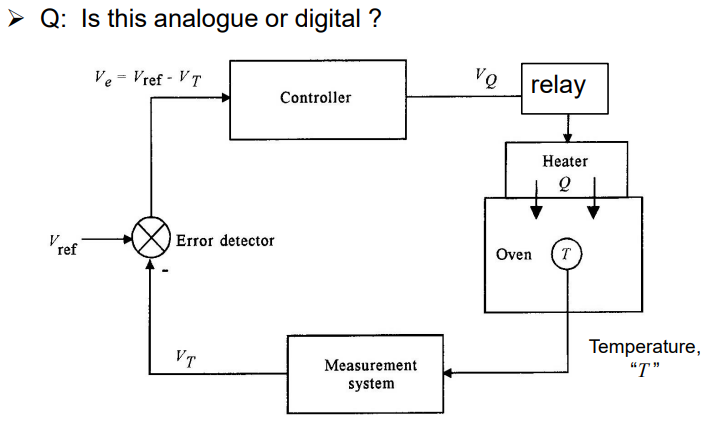
Page 28: ON/OFF Control Systems
Control levels: V(Q) is either 0% or 100% (0 or max)
Example: Thermostatic heater - heat or no heat (leave to cool off)
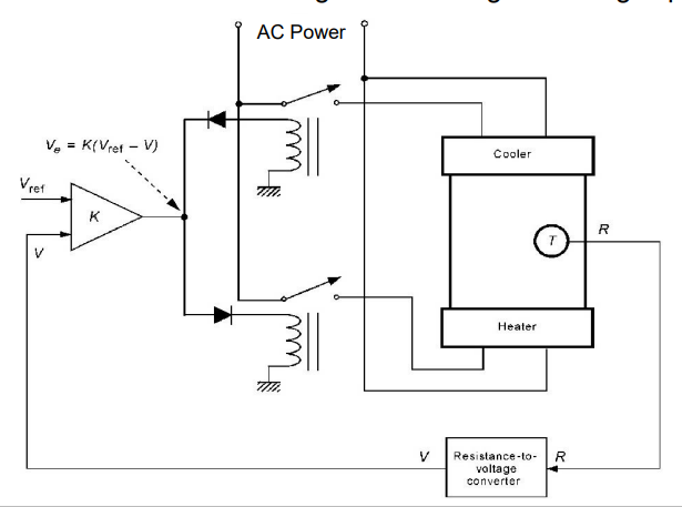
Page 29: Bi-directional ON/OFF Control Systems
Can heat, cool, or do neither
No variation of the degree of heating or cooling is possible.
Three input efforts: 1. Max. heating 2. No effort 3. Max. cooling
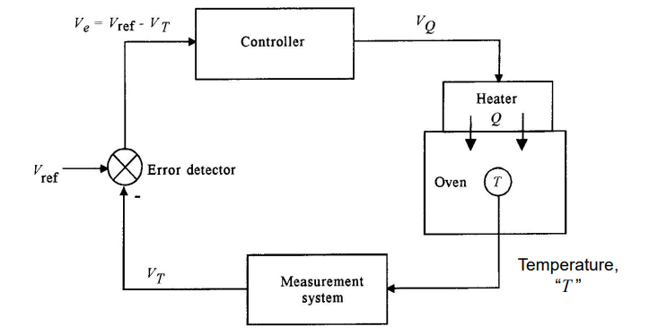
Page 30: Analog Control Systems
This control system allows continuous variation of the controlling input variable (such as heat input Q) as a function of error.
V(Q) and heater power Q can assume any value between 0% and 100%
Page 31: Digital Control System: Supervisory Control
In this control system the computer monitors measurements and updates reference values, but the loops are still analog in nature.
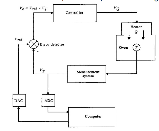
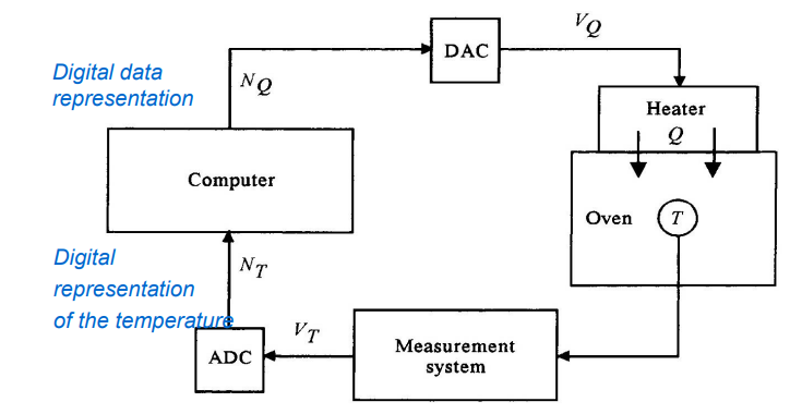
Page 32: Digital Control System: Direct Digital Control (DDC)
The direct digital control system lets the computer perform the error detection and controller functions.
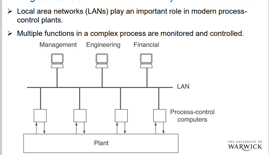
Page 33: Digital Control: Network Control Systems
Role: Manage complex processes via local area networks (LANs)
Page 34: Digital Control: Programmable Logic Controllers (PLCs)
Digital Control: Programmable Logic Controllers
Programmable Logic Controllers (PLCs) are self-contained microcomputers that are optimised for industrial control.
They consist of one or more processors together with power supply and interface circuitry.
A range of input and output modules are available to allow the units to be used in a range of situations.
Facilities are also provided for programming and for system development
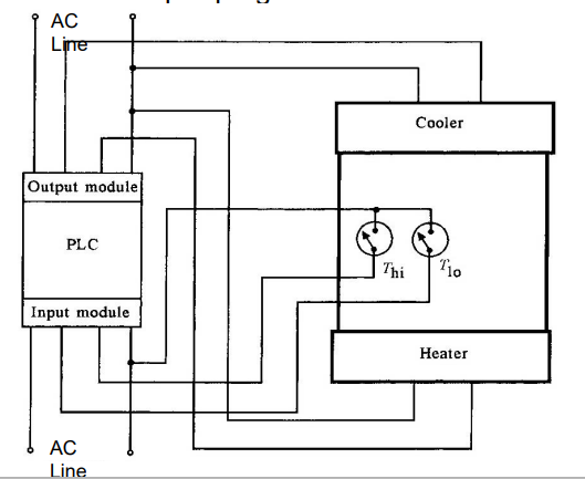
Page 35: Digital Control: PLC Characteristics
Evolution from ON/OFF control; permits time-based programming
In this case the heater and cooler are either ON or OFF. ➢ The PLC can also be pre-programmed in time.
Page 36: Conclusion
Process Control types: Open-loop, closed-loop
Key requirements: Stability, optimal regulation
Analogue, digital, hybrid systems; ON/OFF control is a basic method; PLCs are critical in modern applications
A programmable logic controller (PLC) is a self-contained microcomputer that is optimised for industrial applications, even though originally it was designed to control discrete-state (ON/OFF) systems
NOTEBOOK NOTES
Briefing Document: Process Control and Operational Amplifiers
I. Introduction
This document summarizes key concepts from three lecture excerpts focusing on process control systems and operational amplifiers (op-amps) for instrumentation and signal conditioning. The first lecture introduces fundamental process control concepts and system evaluation. The second delves into op-amp fundamentals and various circuit applications. The third outlines practical signal conditioning principles and design.
II. Process Control Systems (Lecture 1)
A. Core Concepts:
Definition of Control: "Control is the process of altering the performance of a system." This alteration aims for consistency in mass production within continuously operated processes.
Reasons for Control: Systems often don't behave as desired. "Because systems often do not consistently behave the way we would like them to behave." Control mechanisms are implemented to correct this behavior.
Objectives of Control:Regulation: Maintaining a selected output variable at a constant value, despite disturbances. Example: liquid level control in a tank.
Tracking: Forcing an output variable to follow a variable setting or reference value.
Sequencing: Ensuring events occur in a specific order (time- or event-driven). Example: liquid mixing operations in tanks.
Importance of Process Control: "Small changes in a process can have a large impact on the end result." Thus, tight control over variables like proportions, temperature, and flow is crucial for consistent quality, minimized waste, and safety.
Basic Objective: "In the process control, the basic objective is to regulate the value of some quantity, i.e. to maintain that quantity at a desired value, regardless of external influences." Control aims for predictable, stable operations within acceptable variation.
Evolution of Control: Initially performed by humans, control systems have evolved to incorporate machines, electronics, and computers for automatic operation.
B. Process Control Variables:
The lecture lists several variables that are commonly controlled, including:
Pressure
Flow rate
Level
Temperature
Density
pH
Liquid interface
Mass
Conductivity
C. Key Components of Process Control Systems:
Sensors/Transducers/Transmitters: Provide information about the process.
Actuators (Motors, Pumps, Valves, Heaters): Manipulate material or energy.
Controllers: Regulate the process based on sensor data and setpoints.
Interface elements: Facilitate interaction between components and the user.
Setpoint: A desired value for a process variable, which is to be maintained within precise limits.
D. Types of Control Systems:
Servomechanisms: Control a system's position or movement (e.g., robotic arm). The focus is on following a varying reference rather than maintaining a constant value.
Discrete-State Control Systems: Control a sequence of events (e.g., filling and mixing tanks). Events are either on or off, often implemented with Programmable Logic Controllers (PLCs).
E. Open-Loop vs. Closed-Loop Control:
Open-Loop Control: The controlling input is not influenced by the output. It relies on pre-calculated settings. The output can deviate from the expected if the object or environment changes. Examples include a timed sprinkler and a basic electric heater. "Controlling input is not influenced by the output."
Closed-Loop Control: The controlling action is influenced by the output. Feedback from the process is used to adjust the input, minimizing error and stabilizing the process. Examples are a thermostat-controlled heater, rain-sensor controlled sprinkler, and cruise control. "Controlling action IS influenced by the output!"
F. Control System Evaluation:
Objectives:Stability: The control system must be stable.
Steady-State Regulation: Minimum error between the setpoint and actual output at steady state. "The best possible steady-state regulation means that the steady-state error (e) should be at a minimum."
Transient Regulation: Fast response and minimized disturbance from rapid changes. "The transient regulation specifies how the control system reacts to a sudden change or large variation of some process variable..."
Tuning: Adjusting a control loop for optimal control.
Response Types:Damped (Aperiodic) Response: Error approaches zero without oscillation.
Cyclic Response: Output variable oscillates around the setpoint. Evaluation involves measuring overshoot, decay rate, rise time, and settling time.
Tuning Criteria:Minimum Area: Minimize the net area under the error-time curve.
Quarter Amplitude: Ensure each oscillation peak's amplitude is a quarter or less than the preceding peak.
G. Analog vs. Digital Processing
Analog Data: Continuous variation between a variable and its representation. "There is a smooth and continuous variation between representation of a variable value b and the value itself c."
Digital Data: Variable represented by discrete binary numbers (bits), and numbers are represented in terms of binary digits (i.e. bits, “1” or “0”).
Data Conversions:
Analog-to-Digital Converters (ADCs) convert analog signals (e.g. from sensors) to digital representations.
Digital-to-Analog Converters (DACs) convert digital control signals to analog outputs for actuators.
H. Types of Digital Control Systems:
ON/OFF Control: The control effort is either at 0% or 100% (e.g. simple thermostatic heater).
Bi-directional ON/OFF: System can heat, cool or do neither.
Supervisory Control: Computer monitors and adjusts setpoints but underlying loops are analog.
Direct Digital Control (DDC): Computer directly handles error detection and controller functions, replacing analog circuitry.
Network Control Systems: Uses LANs to monitor and control multiple functions in a complex process.
Programmable Logic Controllers (PLCs): Self-contained microcomputers optimized for industrial control with input and output modules.
III. Operational Amplifiers (Op-Amps) (Lecture 2a)
A. Op-Amp Basics
Ideal vs. Real Op-Amps: Real op-amps have limitations (e.g., finite gain, input impedance, output impedance).
Key Characteristics of Real Op-Amps:High differential gain (over 100,000)
Very high input resistance (around 10 MΩ)
Low output resistance (between 10 and 50 Ω)
Operation with supply voltages (e.g. +15V and -15V).
In the linear regime V+ and V- are at the same potential.
B. Common Op-Amp Circuits
Voltage Follower (Buffer): Output voltage equals input voltage. Provides high input impedance and low output impedance. "the voltage at the output is the same as at the input voltage."
Inverting Amplifier: Inverts the input signal and can have gain or attenuation.
Non-Inverting Amplifier: Provides a gain greater than one.
Inverting Summing Amplifier: Adds two or more input voltages. "for adding two or more applied input voltages."
Differential Amplifier: Amplifies the difference between two input voltages. "subtracts one input voltage signal from another and amplifies the difference."
Voltage-to-Current Converter: Converts input voltage to output current.
Current-to-Voltage Converter: Converts input current to output voltage.
Integrator: Output voltage is the integral of the input voltage.
Differentiator: Output voltage is proportional to the derivative of the input voltage.
Linearization Circuits: Uses nonlinear feedback devices (diodes) to linearize the op-amp behaviour.
Stabilising Circuits: Provides a fixed output voltage even as the input voltage varies.
C. Concept of Loading
"The loading of one circuit by another circuit is one of the most important issues/problems in analog signal conditioning." Loading occurs when the output of one circuit is connected to the input of another circuit and their impedances interact.
D. Instrumentation Amplifiers:
Combines differential amplification with high input impedance (voltage followers) to avoid loading issues.
Allows adjustable gain using a single resistor (RG).
E. Comparators:
A 1-bit comparator circuit has a high-low output based on a threshold value.
IV. Op-Amps for Signal Conditioning (Lecture 2b)
A. Aims of Signal Conditioning:
Matching sensor output to the next stage of electronics in terms of signal range and offset.
Preventing sensor loading.
Allowing range and offset adjustments.
Filtering out noise spikes in the sensor signal.
Linearizing non-linear sensor outputs. "The most common task is to match the sensor’s output to the next stage of electronics"
B. Design Guidelines:
Define Measurement Objectives: Parameter, range, accuracy, linearity, speed of change, noise.
Select a Sensor: Based on output type, transfer function, time response, range, and power requirements.
Design Signal Conditioning: Taking into account variable type (voltage or current), input and output ranges and impedances.
C. Example: Temperature Sensor Conditioning:
Problem: Converting a 20-250 mV signal (0-115°C) to a 0-5V range for a D/A converter. The signal needs to be high input impedance to prevent loading.
Solution: Uses a differential amplifier circuit with appropriate gain and offset adjustment. The linear equation "y = m x + b" is used to calculate the required transfer function.
Steps:Define the transfer function using the linear (straight-line) equation .
Choose appropriate circuit structure (differential amplifier and buffer).
Achieve the required gain using standard resistor values (E12 series). "The standard resistor values in E12 series are: 10, 12, 15, 18, 22, 27, 33, 39, 47, 56, 68, 82..."
Set the required reference voltage for offset adjustment, in this example with a Zener diode. "a Zener diode provides a stable low voltage. Even if the V1 changes, the Vz remains practically constant."
V. Conclusion
These lectures provide a comprehensive overview of process control principles and the use of op-amps for signal conditioning in instrumentation. From basic control strategies to complex circuit design, these resources are essential for understanding how to measure, manipulate, and regulate physical processes. The knowledge of both control systems and op-amp circuits is fundamental for developing effective, reliable industrial control systems. "Operational amplifier is a building block" in many analog electronic circuits.