Every Graph to Know for AP Macroeconomics
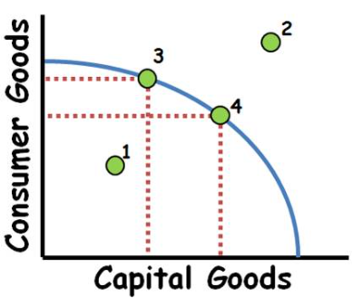
Production Possibilities Curve
Point 1 → Inefficient Use of Resources (but still possible to produce):
This refers to a point inside the Production Possibility Curve (PPC). The PPC shows the maximum combination of two goods that can be produced with the available resources and technology. If production is inside the PPC, resources (like labor, capital, or raw materials) are not being fully utilized—meaning there’s some level of inefficiency. However, even though this point represents underutilized resources, it is still feasible to produce here.
Point 2 → Scarcity Limits Production without New Resources (trade may help):
Points outside the PPC represent a level of production that is currently impossible with the existing resources. Scarcity means we have limited resources, so producing beyond the curve isn’t achievable unless new resources become available. Another way to reach this level of production is through trade, which allows a country to acquire goods it can't produce on its own due to resource constraints.
Points 3-4 → Increasing Opportunity Costs (if the PPC is concave):
The PPC’s shape can reflect opportunity costs. If the curve is concave (bowed outwards), it shows increasing opportunity costs, meaning that as production of one good increases, the resources that are redirected toward that good are less and less suited to it.
For example, if you're moving resources from producing consumer goods to making heavy machinery, some resources (like highly skilled labor) are better suited to consumer goods and less adaptable to machinery. This mismatch raises opportunity costs.
Constant Opportunity Costs (straight-line PPC): If the PPC is a straight line, opportunity costs remain constant. This happens when resources are equally adaptable for producing both goods. In other words, every unit of a good given up results in a fixed amount of the other good being produced.
Shifts in the PPC:
Outward Shift (growth): If there’s an increase in resource quantity (like finding new mineral reserves) or improvements in resource quality (like better-skilled labor) or technology, the PPC shifts outward. This indicates economic growth, allowing more production of both goods.
Inward Shift (decline): A decrease in the quantity or quality of resources, like from a natural disaster or depletion of resources, shifts the PPC inward. This represents a loss in production capacity, limiting how much of both goods can be produced.
Demand and Supply
Law of Demand
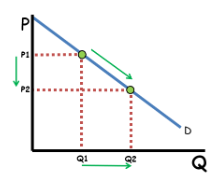
The law of demand is a fundamental principle in economics that states: if all other factors remain constant (ceteris paribus), an increase in the price of a good or service will lead to a decrease in the quantity demanded. Similarly, a decrease in price will lead to an increase in quantity demanded.
This relationship is typically inverse: as price goes up, people buy less of the good, and as price goes down, people buy more. This happens because higher prices make the good less affordable or attractive, while lower prices make it more appealing.
Movement Along the Demand Curve:
The demand curve is a graphical representation of the relationship between price and quantity demanded. When we say "movement along the demand curve," we mean that changes in quantity demanded are caused by changes in the good’s price, not by changes in other factors.
For example, if the price of a product like apples rises, people will buy fewer apples, moving up along the demand curve to a point with a higher price and lower quantity. Conversely, if the price drops, people will buy more apples, moving down along the demand curve to a point with a lower price and higher quantity.
Price vs. Demand vs. Quantity Demanded:
It’s crucial to distinguish between demand and quantity demanded, as they refer to different concepts:
Quantity Demanded is the specific amount of a good that people are willing to buy at a particular price, represented by a single point on the demand curve.
Demand refers to the entire relationship between prices and the quantity demanded at each price level, represented by the entire demand curve.
A change in price affects only the quantity demanded (moving along the same demand curve), not the demand itself. Therefore, when price changes, it doesn’t create a new demand curve; it simply changes the quantity at a particular point on the existing curve.
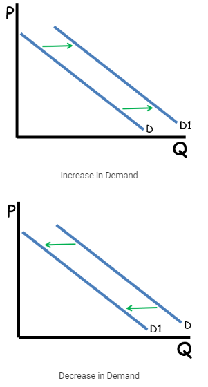
In contrast, changes in factors other than price (like consumer income, preferences, or the price of related goods) shift the entire demand curve. This means people would demand different quantities at all price levels.
Other factors besides price can lead to a change in demand, meaning a change in the quantity demanded at every price level. These factors cause the entire demand curve to shift—shifts to the right represent an increase in demand, while shifts to the left represent a decrease. These factors are known as non-price determinants of demand.
Non-Price Determinants of Demand:
Consumer Tastes and Preferences:
Consumer tastes can change due to trends, advertising, or cultural shifts. When a product becomes popular or “in style,” demand for it increases, causing a rightward shift in the demand curve. Conversely, when a product goes out of style or loses appeal, demand decreases, shifting the curve leftward.
For example, if a new fitness trend makes running popular, the demand for running shoes may increase, shifting the demand curve to the right. Later, if the trend fades, demand may fall, shifting the curve back to the left.
Market Size (Number of Consumers):
The size of the market, or the number of consumers, also impacts demand. When the number of consumers increases, such as from population growth or entry into new markets, the demand curve shifts to the right. A decrease in the number of consumers will shift the curve to the left.
For instance, if a city experiences a population boom, the demand for housing and related goods (like furniture) may increase. Conversely, in an area with a declining population, demand for these goods may decrease.
Prices of Related Goods:
Related goods affect demand based on their relationship as substitutes or complements.
Substitutes: A substitute is a product that can be used in place of another. When the price of a substitute rises, demand for the good in question increases, causing a rightward shift. Conversely, if the substitute's price falls, demand for the original good decreases, shifting the curve left.
For example, if ice cream becomes more expensive, people may buy more frozen yogurt instead, increasing demand for frozen yogurt.
Complements: A complement is a product that is used together with another good. When the price of a complement increases, the demand for the related good decreases, shifting the curve left. When the price of the complement decreases, demand for the related good increases, shifting the curve right.
For instance, if the price of ice cream increases, people might buy less hot fudge to go with it, decreasing demand for hot fudge.
Changes in Income:
Income changes can shift demand differently depending on whether a good is classified as a normal or inferior good:
Normal goods: When income rises, demand for normal goods increases (rightward shift), while a decrease in income lowers demand (leftward shift).
For example, Nike shoes are a normal good; if consumer income rises, people will likely buy more Nike shoes, increasing demand.
Inferior goods: Demand for inferior goods decreases as income rises and increases as income falls.
For example, generic or store-brand cereal might be considered an inferior good. If people’s incomes rise, they might buy less store-brand cereal and more premium brands, reducing demand for the store-brand cereal.
Expectations of the Future:
Consumer expectations about future prices or income can affect current demand. If consumers expect a price increase in the future, they may buy more of the product now, shifting the demand curve to the right. Conversely, if they expect prices to drop, they may hold off on purchasing, shifting the curve to the left.
For instance, if consumers expect gas prices to rise next month, they may fill up their tanks now, causing a temporary increase in current demand for gas.
Demand curves slope downward for three main reasons:
Income Effect: When prices drop, consumers' purchasing power increases, allowing them to buy more. For example, if candy bars drop from $1 to $0.50, a $10 income can buy 20 bars instead of 10. Conversely, when prices rise, purchasing power falls.
Substitution Effect: As the price of a good rises, consumers switch to cheaper alternatives. For instance, if frozen yogurt becomes expensive, people may buy ice cream instead. Lower prices encourage more purchases of the good itself over substitutes.
Diminishing Marginal Utility: The additional satisfaction (utility) from consuming each extra unit of a good decreases. So, as prices rise, consumers find fewer units worth buying because each unit is valued less.
Supply
Law of Supply
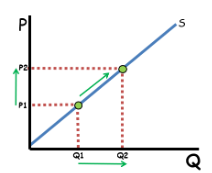
The law of supply states that, all other factors being equal (ceteris paribus), there is a direct relationship between the price of a good and the quantity supplied by producers. Specifically:
Direct Relationship between Price and Quantity Supplied:
When the price of a good increases, producers are more willing to supply more of that good. Higher prices make it more profitable for businesses to produce and sell the goods, so they allocate more resources toward its production, increasing the quantity supplied.
Conversely, when the price of a good decreases, it becomes less profitable to produce, so businesses reduce the quantity they are willing to supply. Lower prices may not cover production costs as well, so producers pull back on the quantity they offer.
Movement Along the Supply Curve:
A change in the price of the good itself causes a movement along the supply curve, which means that only the quantity supplied is changing. For example, if the price of apples goes up, farmers may supply more apples, moving to a higher point on the same supply curve. If the price falls, they will supply fewer apples, moving to a lower point.
This is different from a change in supply, which would involve the entire curve shifting.
Difference Between Supply and Quantity Supplied:
Supply refers to the overall relationship between price and the amount producers are willing to supply at each price point; this relationship is represented by the entire supply curve.
Quantity Supplied is the specific amount offered for sale at a particular price, represented by a single point on the supply curve.
A change in the good’s price affects only quantity supplied (causing movement along the curve) rather than supply itself. To change the overall supply, a non-price factor (like production costs or technology) would need to shift the entire curve.
Non-Price Determinants of Supply
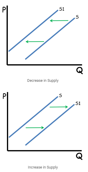
The six main non-price determinants of supply, also known as “supply shifters,” affect the entire supply curve, shifting it either to the right (an increase in supply) or to the left (a decrease in supply). Here’s how each of these shifters works:
Prices of Resources or Inputs:
When the costs of production inputs (like labor, raw materials, or machinery) change, supply is directly impacted.
An increase in resource prices makes production more expensive, leading to a decrease in supply (leftward shift). Conversely, a decrease in resource prices reduces costs, increasing supply (rightward shift).
For example, if baker wages rise, producing cakes becomes more costly, so the supply of cakes decreases. Alternatively, if the price of sugar drops, candy producers can afford to produce more, increasing candy supply.
Government Tools:
Government policies can affect production costs and incentives, influencing supply.
Taxes on production increase costs, decreasing supply (leftward shift).
Subsidies are government payments to producers that lower production costs, increasing supply (rightward shift).
Regulations may also impose additional costs or restrictions, generally leading to a decrease in supply.
For example, a subsidy for electric car manufacturers would increase the supply of electric cars, while stricter environmental regulations may reduce supply if they add compliance costs.
Competition (Number of Sellers):
The number of firms producing a good impacts overall supply.
When more sellers enter the market, total supply increases (rightward shift). When firms exit, supply decreases (leftward shift).
For example, if new coffee shops open in a city, the overall supply of coffee increases. If many close down, the supply decreases.
Technology:
Advances in technology improve production efficiency, allowing producers to supply more at the same cost, which shifts the supply curve to the right.
For example, automated machinery in factories can increase the output of goods without raising costs, increasing overall supply.
Prices of Other Goods:
Producers may shift resources to produce goods with higher potential profit, affecting the supply of other goods.
If the price of a substitute good (like corn) rises, farmers might allocate more land and resources to corn, reducing the supply of other crops like wheat.
This reallocation leads to a leftward shift in the supply of wheat as resources move toward corn production.
Producer Expectations:
Producers’ expectations about future prices or market conditions can influence current supply decisions.
If producers expect prices to rise in the future, they might increase production now to maximize potential profits (rightward shift). Conversely, if they expect lower prices, they might reduce current production.
For instance, if farmers expect grain prices to rise due to future demand, they may increase grain production now, shifting the supply of grain to the right.
Equilibrium in Supply and Demand
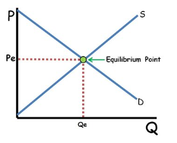
Equilibrium is the price where quantity supplied equals quantity demanded. Market forces drive prices toward this balance.
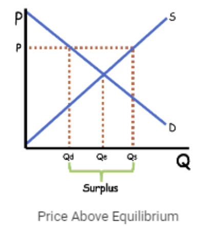
Above equilibrium: A surplus occurs, where quantity supplied exceeds quantity demanded. Suppliers lower prices to eliminate the surplus, increasing quantity demanded and decreasing quantity supplied until equilibrium is reached.
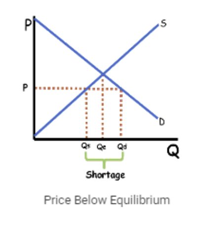
Below equilibrium: A shortage occurs, where quantity demanded exceeds quantity supplied. Suppliers raise prices to eliminate the shortage, decreasing quantity demanded and increasing quantity supplied until equilibrium is reached.
Shifts in supply and demand affect equilibrium price and quantity:
Increase in demand: Both equilibrium price and quantity increase.
Decrease in demand: Both equilibrium price and quantity decrease.
Increase in supply: Equilibrium price decreases, and quantity increases.
Decrease in supply: Equilibrium price increases, and quantity decreases.
Double Shift
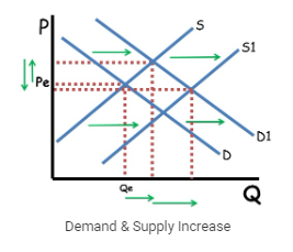
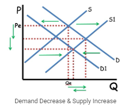
When both supply and demand curves shift simultaneously, the effects on equilibrium price and quantity can be complicated. Here's how double shifts work:
Same Direction (both supply and demand increase or decrease):
Price is indeterminate: An increase in demand pushes price up, while an increase in supply pushes price down. Since both forces act in opposite directions on price, the overall effect on price depends on which shift is stronger, making it impossible to predict the direction of the price change.
Quantity increases: Both shifts increase the equilibrium quantity, as both increased demand and increased supply lead to a higher quantity in the market.
Opposite Directions (one curve shifts up, the other down):
Quantity is indeterminate: When one shift increases quantity (like an increase in demand) and the other decreases quantity (like a decrease in supply), the overall effect on quantity is unclear. We can’t predict whether equilibrium quantity will rise or fall because it depends on the strength of each shift.
Price is determined: The effect on price is clearer. For example, if demand increases while supply decreases, price will rise because both shifts push the price up.
Aggregate Supply and Aggregate Demand (AS/AD)
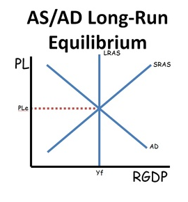
The AS/AD (Aggregate Supply/Aggregate Demand) graph is a key tool in macroeconomics that represents the entire economy and illustrates the three major macroeconomic goals: full employment, price stability, and growth.
Axes:
Y-axis (Price Level): This represents the average price level for all goods and services in the economy, often measured by the GDP deflator or Consumer Price Index (CPI).
X-axis (Real GDP): This measures the total output of the economy, adjusted for inflation, and represents the economy’s National Income (also referred to as Y). Higher Real GDP generally means more employment and lower unemployment.
Aggregate Demand (AD):
Downward Sloping Curve: The AD curve shows the inverse relationship between the price level and Real GDP.
Wealth Effect: As the price level rises, the real value of wealth falls, leading to reduced consumption.
Interest Rate Effect: Higher prices lead to higher nominal interest rates, reducing investment spending.
Net Export Effect: As domestic prices rise, exports become more expensive, reducing demand for them.
Shifters of AD: Changes in the components of GDP (Consumption, Gross Investment, Government Purchases, and Net Exports) shift the AD curve:
Rightward shift: An increase in any of these components (e.g., higher government spending or increased consumer confidence).
Leftward shift: A decrease in these components (e.g., reduced investment or exports).
Inflation Types:
Demand-Pull Inflation: When an increase in AD drives up both the price level and output.
Fiscal and Monetary Policy:
Expansionary Fiscal Policy (e.g., tax cuts or increased government spending) shifts AD right.
Contractionary Fiscal Policy (e.g., tax increases or spending cuts) shifts AD left.
Monetary Policy: The Federal Reserve can influence AD by changing the money supply. Increases in the money supply lower interest rates and shift AD right, while reducing the money supply raises interest rates and shifts AD left.
Short-Run Aggregate Supply (SRAS):
Upward Sloping Curve: The SRAS shows a positive relationship between price levels and Real GDP in the short run. As prices increase, businesses are willing to produce more because input costs (like wages) are "sticky" and don’t immediately adjust.
Shifters of SRAS:
Changes in resource prices (especially wages).
Productivity improvements.
Inflation expectations (higher expected inflation increases costs, shifting SRAS left).
Government regulations and taxes on businesses (tax increases shift SRAS left).
Cost-Push Inflation: A leftward shift of SRAS due to rising production costs (such as higher wages or input prices), causing both inflation and reduced output (stagflation).
Long-Run Aggregate Supply (LRAS):
Vertical Curve: In the long run, the LRAS is vertical at full employment output (Yf), meaning the economy’s potential output is independent of the price level.
This is because, over time, wages and resource prices adjust to changes in the price level, ensuring the economy produces at its full employment output.
Shifters of LRAS: Anything that affects the Production Possibilities Curve (PPC)—such as changes in the quantity or quality of resources, technological improvements, or productivity—will shift the LRAS.
Rightward shift: Increases in resources or technology boost potential output.
Leftward shift: A decrease in resources or productivity reduces potential output.
Short-Run and Long-Run Equilibrium:
Short-Run Equilibrium: This occurs where SRAS and AD intersect.
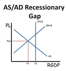
If RGDP is below Yf, the economy is in a recessionary gap, meaning it is producing less than its potential, leading to unemployment.
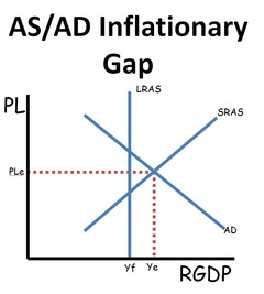
If RGDP is above Yf, the economy is in an inflationary gap, where output is beyond sustainable capacity, causing upward pressure on prices.
Long-Run Equilibrium: In the long run, the economy will naturally adjust to the LRAS (full employment) level:
In an inflationary gap, higher wages and input costs shift SRAS left, reducing output and bringing the economy back to Yf.
In a recessionary gap, lower wages and input costs shift SRAS right, increasing output and restoring full employment.
Fiscal and Monetary Policy can also help speed up this adjustment process by shifting the AD curve.
Loanable Funds Market
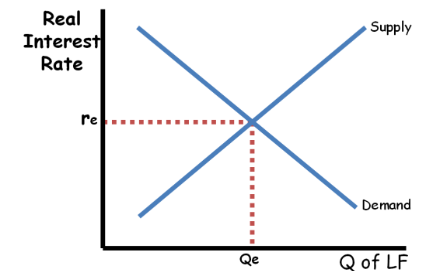
The Loanable Funds Market illustrates how the supply and demand for funds, or loans, determine the real interest rate in an economy. This market is for understanding how investment and savings interact and how interest rates affect economic growth:
Axes of the Loanable Funds Market:
Y-axis (Real Interest Rate, r): This is the "price" of borrowing funds, representing the real interest rate (the nominal interest rate adjusted for inflation). The real interest rate is what lenders earn on their loans after accounting for inflation, and what borrowers must pay to use the funds. The real interest rate affects how much borrowing and lending occurs in the market.
X-axis (Quantity of Loanable Funds): This represents the amount of money available for borrowing and lending in the economy, typically shown as the total amount of funds that consumers and businesses are willing to save and invest.
Supply and Demand in the Loanable Funds Market:
Supply Curve (Savings): This curve represents the amount of money available for borrowing, and it comes from people or entities willing to save their money and lend it out at a given interest rate. The supply of loanable funds increases when interest rates are higher, because higher rates make saving more attractive.
Demand Curve (Investment): This curve represents the amount of money that businesses and other borrowers wish to borrow to invest in projects, such as expanding operations or purchasing capital. The demand for loanable funds is generally higher when the expected return on investment is higher.
Determinants of Loanable Funds Demand:
The demand curve shifts based on factors that change the expected rate of return on investments:
Expected Rate of Return: This is the primary determinant of investment demand. If businesses expect a higher return on their investments, they will demand more loanable funds. If the economy is growing or there are incentives like tax credits or favorable market conditions (e.g., optimism about future growth), businesses are more likely to take out loans.
Bullish sentiment about the economy (positive expectations) increases investment demand.
Bearish sentiment (negative expectations) reduces investment demand.
Determinants of Loanable Funds Supply:
The supply of loanable funds comes from savings, and several factors influence how much people are willing to save and lend:
Consumer Savings:
Changes in Disposable Income: When people have more income, they can save more, increasing the supply of loanable funds. Conversely, lower income reduces savings and the supply of funds.
Other Factors Influencing Savings: Anything that encourages or discourages consumers to save will shift the supply curve. For example, increased confidence in the economy or higher interest rates may encourage people to save more.
Foreign Investment: When foreign investors bring their capital into a country, they increase the supply of loanable funds available for borrowing. This can help lower interest rates and increase investment.
Connection to Economic Growth:
The real interest rate plays a significant role in determining economic growth because it affects investment levels:
High Interest Rates: When interest rates are high, borrowing becomes more expensive. This reduces the quantity of new investment, which can slow capital formation and economic growth.
Low Interest Rates: When interest rates are low, borrowing becomes cheaper, encouraging more investment. This leads to higher capital formation and can boost economic growth.
Fiscal Policy and Loanable Funds:
Fiscal policy, particularly government spending and borrowing, can significantly influence the loanable funds market:
Crowding Out:
When the government runs a deficit (spending more than it collects in revenue), it borrows money by issuing bonds, which increases the demand for loanable funds.
This increased demand for funds raises interest rates, making borrowing more expensive for businesses and consumers. As a result, private investment may be "crowded out" by the government's borrowing.
Expansionary fiscal policy (increased government spending or tax cuts) leads to a higher deficit, increased government borrowing, and higher interest rates, which can reduce private investment and long-term economic growth.
Contractionary Fiscal Policy:
Decreasing the deficit (through lower spending or higher taxes) reduces government borrowing, which lowers interest rates. This can increase private investment, as businesses can borrow at more favorable rates.
Money Market
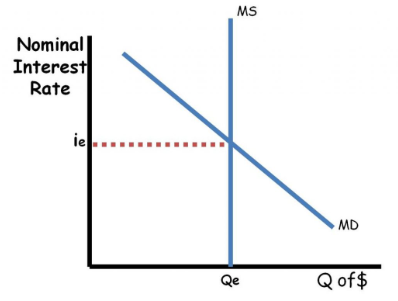
The money market is a model used to show the relationship between the nominal interest rate (the cost of borrowing money) and the quantity of money in an economy. It explains how money supply and demand interact to determine interest rates, and how these rates influence other economic variables, such as investment and aggregate demand.
1. The Money Market Overview:
The money market works like a typical competitive market, but with a few key differences:
Y-axis: The nominal interest rate (denoted as “i”) represents the price of money, which is the interest rate that borrowers must pay to lenders.
X-axis: The quantity of money, which refers to the amount of money in circulation in the economy.
The demand curve in the money market is downward sloping, showing an inverse relationship between the interest rate and the demand for money.
The supply curve is perfectly inelastic (vertical), meaning that the quantity of money does not change based on the interest rate. This is because the money supply is controlled by the central bank.
2. The Demand for Money:
The demand curve for money has two components:
Transaction Demand for Money: This is the demand for money for everyday transactions. It depends on the overall level of economic activity, particularly nominal GDP (the total market value of goods and services in an economy). Any change in GDP or the price level will alter the transaction demand for money.
For example, if nominal GDP increases, people will need more money to facilitate transactions, increasing the demand for money.
Asset Demand for Money: This is the demand for money as a store of value or asset. People hold money because it is liquid and can be used for future transactions, but it does not earn interest (unlike other assets such as bonds or savings accounts).
The opportunity cost of holding money is the interest that could have been earned by saving or investing it elsewhere.
When interest rates are high, the opportunity cost of holding money increases, so people prefer to save or invest rather than hold money, reducing the demand for money as an asset.
When interest rates are low, the opportunity cost of holding money decreases, so more people demand money as an asset.
As a result of the inverse relationship between the nominal interest rate and the quantity of money demanded as an asset, the demand curve is downward sloping. The demand for money shifts when there are changes in factors like GDP, the price level, or people’s desire to hold wealth as money (e.g., during times of economic uncertainty).
3. The Supply of Money:
In a limited reserves system (as is typical in modern economies), the money supply is controlled by the central bank and is perfectly inelastic—it does not change in response to interest rates. Instead, the central bank adjusts the money supply through various monetary policy tools:
Discount Rate: This is the interest rate that banks pay when borrowing money from the central bank. Lowering the discount rate increases the money supply because it becomes cheaper for banks to borrow, which can encourage lending to consumers and businesses.
Reserve Requirement: This is the percentage of deposits that banks are required to keep in reserve and not lend out. Lowering the reserve requirement increases the money supply by allowing banks to lend more of their deposits.
Open Market Operations: This involves the buying and selling of government bonds by the central bank. When the central bank buys bonds, it injects money into the economy, increasing the money supply. Conversely, selling bonds reduces the money supply.
4. Nominal Interest Rates and Bond Prices:
Interest rates and bond prices are inversely related. When interest rates rise, the price of existing bonds falls, and when interest rates fall, the price of existing bonds rises.
Example: Suppose a bond was issued with a 5% coupon rate (i.e., it pays $50 annually for a $1,000 bond). If interest rates rise to 10%, newly issued bonds will pay $100 annually. In comparison, the older bond with a $50 annual payment becomes less attractive, so its price will fall to $500 to match the new higher yields.
On the other hand, if interest rates fall, the price of older bonds with higher interest payments becomes more attractive, so their price rises.
5. The Money Market’s Connection to Other Models:
The money market has significant effects on other areas of the economy:
In the AS/AD model: When the central bank increases the money supply (e.g., by buying bonds), it lowers nominal interest rates. Lower interest rates make borrowing cheaper, which increases investment. This leads to a rightward shift in the aggregate demand (AD) curve, increasing real output and reducing unemployment in the short run.
If the central bank raises interest rates (e.g., by selling bonds), investment decreases, leading to a leftward shift in the AD curve. This results in lower output and higher unemployment.
In the long run: The money supply affects aggregate demand and real output. In the short run, an increase in the money supply can shift the AD curve rightward, raising output. However, in the long run, wages and prices adjust to the higher money supply. The short-run aggregate supply (SRAS) curve may shift leftward due to higher input costs (wages), bringing the economy back to its long-run potential output, but with higher prices (inflation).
In the Foreign Exchange Market: When the interest rate in a country rises, it attracts foreign investment seeking higher returns. Foreign investors will need to purchase the country’s currency, increasing the demand for that currency and causing it to appreciate. This is an important concept in the global financial markets, as currency fluctuations affect trade balances and capital flows.

Phillips Curve
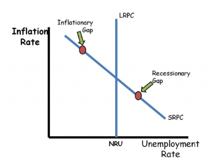
1. Axes of the Phillips Curve:
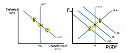
Y-axis (Inflation Rate): This represents the inflation rate in the economy, which is the percentage change in the general price level over time. This is similar to the price level in the AS/AD model. When inflation increases, the overall price level in the economy is rising.
In the context of the Phillips Curve, inflation is often measured by the percentage increase in prices, like the Consumer Price Index (CPI). A higher inflation rate means a faster rise in prices.
X-axis (Unemployment Rate): This represents the unemployment rate, or the percentage of people who are actively looking for work but unable to find a job. The Phillips Curve suggests that there is an inverse relationship between inflation and unemployment in the short run.
In contrast to the AS/AD model, where the X-axis shows Real GDP (which relates to the total output of the economy and thus employment), the Phillips Curve directly shows how inflation and unemployment are related.
2. Short-Run Phillips Curve (SRPC):
The SRPC is a downward sloping curve that shows an inverse relationship between inflation and unemployment in the short run. This means:
When unemployment decreases, inflation tends to increase (and vice versa).
This relationship can be explained by the concept that when unemployment is low, labor is more scarce, which leads to higher wages. Higher wages can lead to higher production costs, which businesses pass on to consumers in the form of higher prices (inflation).
Movement along the SRPC:
When there is a demand shock, the aggregate demand (AD) curve shifts, causing changes in the unemployment rate and inflation rate. For example:
Inflationary gap (rightward shift in AD): When demand increases in the economy, it leads to more output and employment, but also higher inflation. This would result in movement upward along the SRPC, indicating a decrease in unemployment and an increase in inflation.
Recessionary gap (leftward shift in AD): When demand decreases, unemployment increases, and inflation falls, causing movement downward along the SRPC.
SRPC Shifters:
Supply Shocks: These are sudden changes in the availability of key resources (e.g., oil price shocks or natural disasters) that affect production costs. A negative supply shock (e.g., an increase in oil prices) shifts the SRAS curve to the left and also shifts the SRPC to the right (higher inflation and higher unemployment). A positive supply shock shifts the SRAS curve to the right and shifts the SRPC to the left (lower inflation and lower unemployment).
Inflation Expectations: If workers and businesses expect inflation to rise in the future, they will adjust their wages and prices upward in anticipation. This will cause the SRPC to shift upward (right), leading to higher inflation at any given level of unemployment. Conversely, if inflation expectations decrease, the SRPC shifts downward (left).
3. Long-Run Phillips Curve (LRPC):
In the long run, there is no trade-off between inflation and unemployment. The LRPC is a vertical curve at the Natural Rate of Unemployment (NRU), also known as the Non-Accelerating Inflation Rate of Unemployment (NAIRU). This suggests:
The economy can return to its natural rate of unemployment regardless of the inflation rate.
The NRU is not zero; it includes structural unemployment (mismatch between workers' skills and job requirements) and frictional unemployment (temporary unemployment while transitioning between jobs).
Changes in the NRU can shift the LRPC. For example:
If structural unemployment increases (due to technological changes or a mismatch in job skills), the NRU increases, and the LRPC shifts to the right.
If structural unemployment decreases (due to improved education or better job matching), the NRU decreases, and the LRPC shifts to the left.
4. Short-Run vs Long-Run Phillips Curve:
Short-Run: The short-run Phillips Curve suggests that policymakers can trade off between inflation and unemployment—i.e., by accepting higher inflation, they can reduce unemployment, and vice versa.
Long-Run: In the long run, however, inflation does not affect unemployment. The economy will always return to its natural rate of unemployment, regardless of inflation, because wages and prices adjust over time. This is why the LRPC is vertical at the NRU.
5. Expectations and the Phillips Curve:
The intersection of the SRPC and LRPC represents the expected inflation rate. In the short run, the actual inflation rate can be higher or lower than expected based on demand shocks (inflationary or recessionary gaps).
Inflationary Gap: If the economy is operating above its potential (due to an increase in aggregate demand), the actual inflation rate will be higher than expected, and the economy will be above the natural rate of unemployment.
Recessionary Gap: If the economy is operating below its potential (due to a decrease in aggregate demand), the actual inflation rate will be lower than expected, and the economy will be below the natural rate of unemployment.
6. Policy Implications:
Monetary and Fiscal Policies: In the short run, governments and central banks can influence inflation and unemployment through monetary policy (adjusting the money supply) or fiscal policy (changing government spending and taxation). However, in the long run, these policies have limited impact on unemployment, as the economy gravitates toward its natural rate.
Inflation Expectations: If inflation expectations are anchored (i.e., people believe inflation will remain stable), then the short-run trade-off between inflation and unemployment may be more predictable. If expectations are volatile, policymakers face more challenges in managing inflation and unemployment.
Foreign Exchange Market
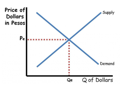
The Foreign Exchange (Forex) Market is where currencies are bought and sold, with the price of one currency relative to another determined by the exchange rate. NOTE: This explanation uses the US Dollars and Mexican Pesos for consistency, but the principles apply to any two currencies.
Axes of the Foreign Exchange Market:
Y-axis: This axis represents the exchange rate in Pesos per Dollar (also called Pesos/Dollar or the Price of Dollars in Pesos). The exchange rate tells you how much one currency (USD) is worth in terms of another currency (MXN).
When the exchange rate increases (i.e., it takes more Pesos to buy 1 Dollar), the US Dollar appreciates relative to the Mexican Peso.
When the exchange rate decreases (i.e., it takes fewer Pesos to buy 1 Dollar), the US Dollar depreciates relative to the Mexican Peso.
X-axis: This represents the quantity of US Dollars in the foreign exchange market. The demand for US Dollars and the supply of US Dollars in the market are based on various economic factors.
At the point where the demand curve and the supply curve intersect, you get the equilibrium exchange rate and the equilibrium quantity of US Dollars. The equilibrium exchange rate determines the value of the Dollar relative to the Peso, while the quantity represents how many Dollars are being exchanged.
Determinants of Currency Demand:
There are three main factors that influence the demand for a currency (in this case, US Dollars):
Demand for Exports:
When a country's exports increase, foreign buyers need the domestic currency to pay for those exports. For example, if Mexico increases its demand for US goods, Mexican consumers or businesses will need to exchange Pesos for US Dollars. This increases demand for the Dollar and causes the Dollar to appreciate.
Factors influencing export demand include:
Price levels: If US goods are relatively cheaper, foreign demand will increase.
Foreign national income: If foreign countries experience economic growth, they may have more income to purchase foreign goods, increasing demand for the US Dollar.
Tastes and preferences: If foreign consumers like US goods, demand for exports and thus demand for the Dollar will rise.
Interest Rates:
When interest rates in the US rise relative to those in Mexico, foreign investors will seek higher returns by investing in US assets (like bonds, stocks, or other financial products). To do so, they must first purchase US Dollars, increasing demand for the Dollar.
Conversely, if interest rates in Mexico rise relative to the US, foreign investors will demand more Pesos to invest in Mexico, decreasing the demand for Dollars and causing the Dollar to depreciate.
Expected Future Exchange Rates:
If investors expect the Dollar to appreciate in the future, they may increase their demand for Dollars today, anticipating higher returns later.
If they expect the Dollar to depreciate, they may reduce their demand for Dollars, anticipating that they’ll get less value for their Dollars in the future.
Determinants of Currency Supply:
Just as there are factors that determine the demand for a currency, there are also factors that determine the supply of a currency in the foreign exchange market:
Demand for Imports:
When a country (e.g., the US) demands more imports, US consumers or businesses need to exchange US Dollars for foreign currencies (like Mexican Pesos) to pay for those imports. This increases the supply of US Dollars in the foreign exchange market. More imports lead to more supply of Dollars and consequently, the Dollar may depreciate relative to other currencies.
Factors that influence the demand for imports include:
Price levels: If foreign goods are cheaper, the demand for imports will rise.
National income: If US income rises, US consumers may demand more foreign goods, thus increasing the supply of Dollars.
Consumer preferences: If consumers favor foreign goods, this increases the supply of Dollars as they purchase foreign currencies.
Interest Rates:
If interest rates in the US decrease relative to Mexico, foreign investors may move their money to Mexico to seek better returns. To do so, they must sell US Dollars to buy Pesos, thus increasing the supply of US Dollars in the market.
Conversely, if interest rates in Mexico decrease relative to the US, the supply of Pesos will decrease as people in Mexico are less likely to sell Pesos for Dollars.
Expected Future Exchange Rates:
If investors expect the Dollar to depreciate in the future, they may want to sell their Dollars today to avoid losing value later, which increases the supply of US Dollars in the market.
If they expect the Dollar to appreciate, they may hold on to their Dollars, reducing the supply of Dollars in the market.
How Exchange Rates Impact Net Exports (Xn):
Exchange rates have a significant impact on a country’s net exports (Xn = Exports - Imports):
When the US Dollar appreciates, it becomes more expensive for foreign countries to purchase US goods and services. As a result, US exports decrease, and imports become cheaper for US consumers. Therefore, a stronger Dollar tends to decrease net exports (Xn).
When the US Dollar depreciates, US goods and services become cheaper for foreign consumers. This leads to an increase in exports, while imports become more expensive for US consumers. As a result, a weaker Dollar tends to increase net exports (Xn).
In summary:
Stronger Dollar = Decreased exports and Increased imports, leading to a decrease in net exports.
Weaker Dollar = Increased exports and Decreased imports, leading to an increase in net exports.
Special Notes About the Foreign Exchange Market:
Currencies are closely linked in the foreign exchange market. For example, when you exchange US Dollars for Mexican Pesos, you are increasing the supply of US Dollars and the demand for Pesos simultaneously. Similarly, when you exchange Pesos for Dollars, you are increasing the supply of Pesos and the demand for Dollars.
This means the supply of one currency is always linked to the demand for the other currency. When the US Dollar appreciates relative to the Mexican Peso, the Mexican Peso depreciates relative to the US Dollar, and vice versa.
Double Shifts: Since the factors influencing demand and supply for a currency are similar, demand and supply curves often move together. For instance, if the demand for US Dollars increases (e.g., due to higher US exports), this generally reduces the supply of US Dollars as fewer Dollars are available for foreign exchange. This interaction leads to amplified shifts in the exchange rate, and in some cases, the equilibrium quantity of currency exchanged can become indeterminate.
Example: If a country’s exports increase, this shifts the demand for Dollars to the right, which might cause the supply of Dollars to decrease, leading to a stronger Dollar. These complex interactions make exchange rates harder to predict when both demand and supply are shifting at the same time.

Business Cycle
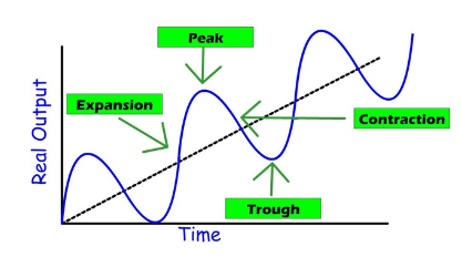
The business cycle refers to the natural fluctuations of an economy through periods of expansion (growth) and contraction (recession). These cycles are an part of a capitalist economy, driven by various economic forces, such as consumer demand, investment levels, and external factors like government policy or global market conditions.
The Three Main Goals of the Economy:
The goals of the economy reflect the desired outcomes for a healthy and sustainable economy, and they guide government policy (fiscal and monetary) efforts to smooth out the business cycle. The three main goals of the US economy are:
Full Employment (4-6% Unemployment):
The goal of full employment is to minimize cyclical unemployment, which is caused by fluctuations in the economy. A fully employed economy means most people who are willing and able to work have jobs, with the remaining unemployment being frictional (temporary transitions) and structural (mismatch of skills and job opportunities).
Unemployment is lowest at the peak of the cycle, when the economy is booming, and highest at the trough, when the economy is in a downturn.
Stable Prices (2% Inflation):
Maintaining price stability is important for preventing inflation from eroding purchasing power and causing uncertainty in the economy. The goal is for inflation to be low and predictable, with a target of approximately 2% annually.
Inflation is highest at the peak of the business cycle when demand outpaces supply, and lowest at the trough when demand is weak and prices may even decrease (deflation).
Growth (2-3% Real GDP Annual Increase):
Economic growth is the expansion of the economy’s total output of goods and services over time, measured by Real GDP (adjusted for inflation). Growth isn’t just about increasing GDP in the short term; it’s about expanding the economy’s potential to produce more goods and services over time.
A healthy economy should have steady growth, usually around 2-3% annually. True economic growth is driven by improvements in productivity, technology, and the availability of resources.
The Four Stages of the Business Cycle:
The business cycle progresses through four stages, each characterized by different economic conditions:
Expansion (Recovery):
This stage is marked by rising economic activity—increasing GDP, falling unemployment, and generally higher demand for goods and services. Businesses invest, hire more workers, and consumers spend more. This leads to further growth in output and wages.
Peak:
The peak represents the point at which the economy is operating at or near its maximum output, with low unemployment and high demand for goods and services. At this stage, inflation tends to be higher because demand exceeds the economy’s capacity to produce goods and services, creating upward pressure on prices.
This period is often referred to as an inflationary gap, where actual GDP is greater than potential GDP. The economy is "overheating," leading to inflation.
Contraction (Recession):
A contraction occurs when the economy slows down, leading to a decrease in output, employment, and income. Businesses may reduce production and lay off workers, while consumer spending decreases. If the contraction lasts for two consecutive quarters (6 months), it is classified as a recession.
During a contraction, unemployment rises, and economic output falls below potential, creating a recessionary gap. The economy may experience deflation, or a reduction in the general price level, as demand weakens.
Trough:
The trough is the lowest point of the cycle, marking the end of the recession and the beginning of a recovery. Economic activity bottoms out, and the economy starts to grow again. Unemployment remains high for some time, but inflation may be low or even negative.
Once the economy begins to recover from the trough, it starts moving toward the long-run equilibrium, where the actual GDP equals potential GDP, and the economy stabilizes.
Indications of the Business Cycle:
To assess the current stage of the business cycle and predict future movements, economists use indicators. These indicators can be categorized as leading, lagging, or coincident indicators, each providing different insights into the economy.
Leading Indicators:
These indicators predict future economic activity and can help anticipate the direction the economy will take. While they are not always accurate, they are useful for forecasting trends. Common leading indicators include:
Business inventories: A large, unexpected increase in inventories (unsold goods) often signals that demand is slowing down. This suggests that businesses might reduce production and employment in the near future, leading to a downturn.
Stock market performance: Stock prices often rise before the economy expands and fall before a contraction.
Consumer confidence: When consumers feel confident about the economy, they tend to spend more, which can indicate future economic growth.
Lagging Indicators:
Lagging indicators provide information about past economic performance. They do not predict future trends but help confirm trends that have already occurred. Common lagging indicators include:
Gross Domestic Product (GDP): GDP is a key measure of economic activity and is reported quarterly. It confirms whether the economy is in a period of expansion or contraction.
Unemployment rate: The unemployment rate is a lagging indicator because it reflects past changes in the labor market. Unemployment often continues to rise even after a recession has ended, as businesses slowly begin to hire again.
Consumer Price Index (CPI): The CPI measures inflation, and it can confirm whether prices are rising (inflation) or falling (deflation) after the fact.
Coincident Indicators:
Coincident indicators occur in real time and provide immediate information about the state of the economy. They rise and fall in line with economic activity. Common coincident indicators include:
Industrial production: The total output of factories, mines, and utilities. It rises during expansions and falls during contractions.
Personal income: Changes in income can provide insight into the health of the economy, as rising wages and employment tend to occur during expansions.
 Knowt
Knowt
