Table of Contents

1. Positive Interactions

2. Ecological Networks

3. Metapopulations & Metacommunities

4. Metapopulations & Variable Environments

5. Evolutionary Community Ecology & Ecological Restoration

Positive Interactions

Interactions can be context dependent

Ant-acacia mutualism can become parasitic: Plants began to decrease their food reward and ants become antagonistic in their behaviour. Slower growth with trees when in the presence of ants.

• Affects communities: Ant increase biomass of acacias. Ants protect them from herbivores (attack), gain benefit of thorns as habitat for young, Ant benefit from habitat in thorns and nectaries as food source. 14x more biomass and 72% survival rate vs. 43% when in the presence of ants.

Desert nurse plants can be facilitators or competitors: plants that shade substrate, decreasing water loss/increase soil fertility. Nurse plants made the benefits in water-stressed environment great for community structure and species richness. After a certain height, they just started competing - competition for nutrients and light.

Mycorrhizal association go from from facilitation to parasitic if soil resources are plentiful: positive seedling-adult interactions shift to negative as seedlings mature to become predators.

Pollinator facilitation: showy plant may bring more visitors to a less showy neighbour, but it also may take away pollinators.

• Type III functional response is good way to keep facilitation. Type II unlikely for pollinators to keep facilitation.

• Most shared pollinator interactions between natives had no effect on plant reproductive success. Exotic species significant negative effect (superior competitors to pollinators).

Anemonefish, damselfish and anemones: anemonefish develop mucus to prevent from being stung by anemone (defense mechanism; food and protection). Anemonefish hide in anemone, and anemonefish cleans anemone and feeds it (food) and defends it from predators.

• Service mutualism

• Interspecific competition stops two species of anemonefish from existing.

• Sea anemones in presence of fish grew faster, reached larger sizes. Larger ones can support damselfish

• Damselfish worse competitor, but competition lightens when anemonefish provide more resources to the anemones.

Mutualist mediated coexistence: Two competing plant species have mutualisms with mycorrhizal fungi. Inferior competitor can be excluded, but if the fungus prefers it they can coexist. Depends on what’s present.

Positive interactions influence abundances and distribution of species: Habitat mutualisms effect abundance of species receiving habitat. Obligate mutualism - distribution of one species dictates the distribution of another species.

Indirect effect: fungi allow plants to exist in areas it couldn’t otherwise, changing the base of the food web. Dominant competitors with reduced performance without mutualism, increasing species richness with weaker competitors doing well.

Cleaner fish: remove parasites from clients (service). fish get food (trophic). Cleaner fish make numbers of fish species and abundances increase. Visits 2300 clients, removing 1220 parasites a day.

Stress gradient hypothesis (SGH): The importance of competition or facilitation interactions differ under different levels of stress. Facilitation more important in stress, competition more important in benign.

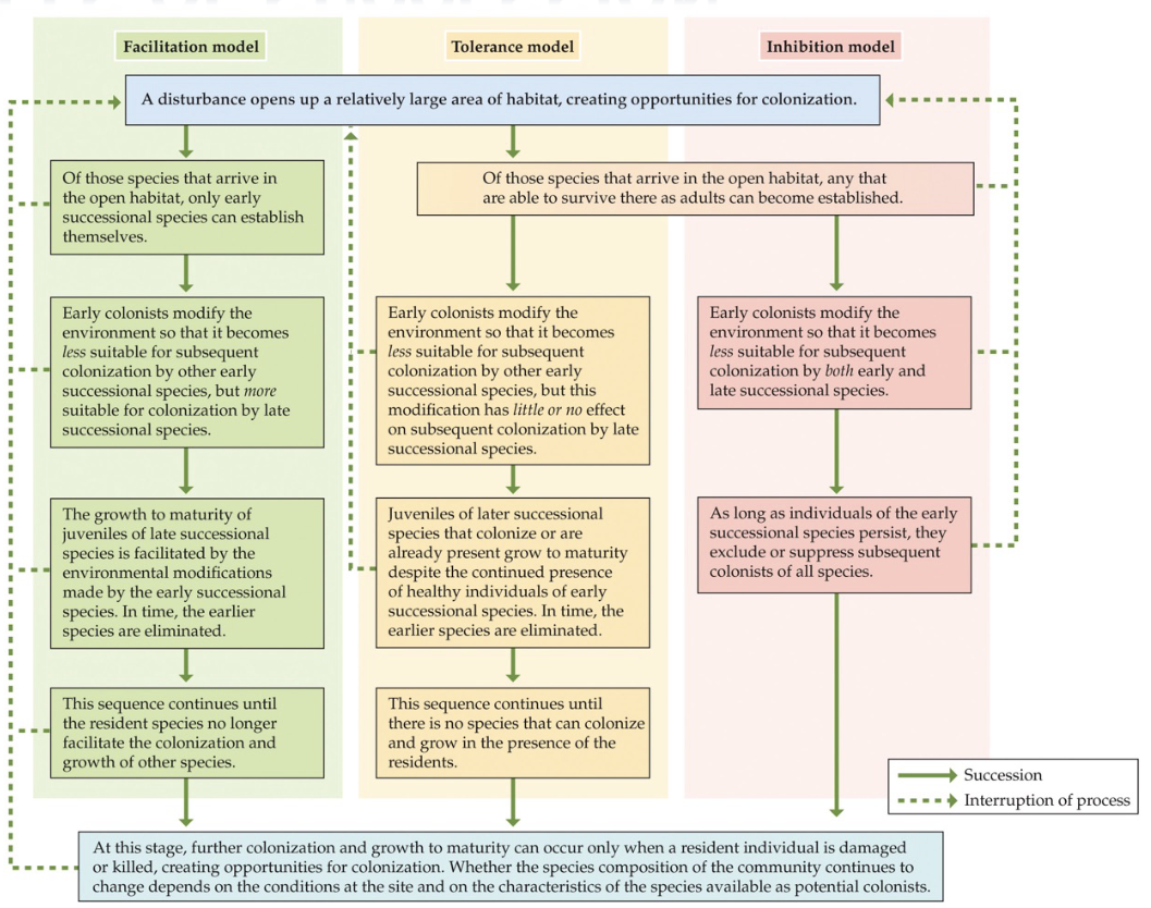
• Primary succession: colonization of newly exposed substrates (e.g. receding glaciers, shorelines, volcanic activity, new islands). Facilitation model shows early successional species being good at colonizing open habitats and dealing with physical stress, but modify environment in ways that benefit later arrivals (facilitation).

RNE: relative neighbour effect - measures effects of neighbours on target species

RNE positive at high elevations: neighbours have positive effect in more stressful environments

RNE negative at low elevations: neighbours have negative effect in less stressful environments.

Ecological Networks

Species represented as nodes, links between nodes represent interactions between species

Food web: focus is on trophic interactions

Host-parasite web: food web that focuses on negative interactions between parasites and their hosts

Herbivory networks: food web that focuses on grazers and their resources

Mutualist web: focus is on interactions that benefit both species

Network topology: pattern of interactions

Interaction webs: includes trophic (vertical) interactions and non-trophic (horizontal) interactions. First level is primary producers (autotrophs), then primary consumers (herbivores), then secondary consumers (carnivores), then tertiary consumers (carnivores/often top predator).

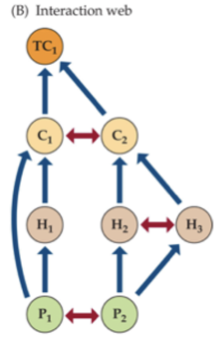
Mutualistic networks show a diagram of species as webs of links between species or functional groups. Pollination and seed dispersal show an important mutualism network. Strength of interaction usually highlighted in thickness of a line

• Topological properties:

  • Connectance: high. number of observed links in networks, expressed as a proportion of the total number of possible links

  • Nestedness: high. specific type of interaction structure in which species with many interactions (generalist) form a core of interacting species. Specialist normally interacts with generalist and not with each other.

  • Modularity: low. Exists when groups of species interact among themselves more than with species from other groups.

• Mutualism may evolve into predictable community structure.

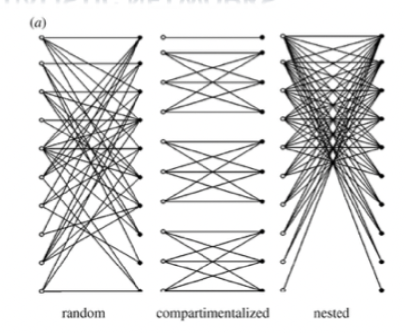
Thebault and Fontaine (2010): compared 34 mutualistic networks (pollination) and 23 trophic networks (herbivory). Mutualistic ones increased in nestedness and connectance. Trophic ones increased in modularity. Both promoted stability. Both differ in topologies, impacting network stability.

Food Chains and Webs

Autotrophs (primary producers): Form organic molecules through the reduction of inorganic carbon (nitrogen, phosphorous) obtained from physical environment.

Hetertrophs (consumers): Obtain organic carbon and other elements needed for growth from other organisms. Can be from autotrophs or others like them. Decomposers are a special class.

There are two types of trophic structure:

1. Food chains: transfer of energy and nutrients through trophic levels, each species exists only at one trophic level in chain

2. Food webs: transfer of energy and nutrients through all traditional predator-prey trophic levels, species can exist in several trophic levels at the same time.

Food chains → transfer of energy and biomass, flow originates from autotroph/primary producers, herbivores are primary consumers, secondary and tertiary are the predators and parasites.

Trophic level: based on number feeding steps to autotrophs

Food webs → shows all predator/prey interactions, does not include information about strength of interactions, species can feed at multiple levels at once, many species are omnivores, idealized webs do not include detritivores, symbionts, nor non-trophic interactions like competition.

Connectedness webs (structural webs): shows all trophic interactions between species but not strength. shown as species or guild at higher trophic levels (less to identify). At lower trophic levels, grouped by broad functional groups. Most webs better resolved at higher levels → lower levels are hard to identify to species level, more numerous, and difficult to quantify in terms of trophic relationship. Show all relationships evenly.

• Green food webs: basal trophic level is autotrophs (fast E channel)

• Brown food webs: basal trophic level is detritus (slow E channel)

• Structural properties: generality (number of species that are prey for a specific predator), vulnerability (numbers of predators a prey species is consumed by).

Energy flow webs: Measures of amount of energy (biomass) moving between species within a food web. Difficult. Some communities fit energy flow, others do not. Is there importance in the energy flow based on how much flows? Show the thickness of arms.

Trophic period: relative amounts of energy or biomass in each trophic level. Terrestrial ecosystems are like a pyramid - energy and biomass periods are similar (close association between energy and biomass). Aquatic ecosystem are inverted because phytoplankton have short lifespans and high turnovers. Lots of energy at base, but like no biomass. Most biomass is at the highest level.

Inverted pyramids are more common where productivity is lowest (open oceans)

Functional webs: focus is on strength of interactions between species within community. Measure strength through removal experiments. Weak interactions are overrepresented in nature and can play a large role in stability food webs.

Parasitism

Parasitism: an interaction in which one organism consumes the tissues or fluids of another organism that it lives on or inside (its host) (-/+)

• parasite attack very few prey over lifetime, consume part of host, do not kill host immediately, form close ties to host, and can trick host into helping them.

Pathogens: parasites that cause disease

Parasitoids: act like parasites at first, but eventually kill their host (so also act like predators)

Parasitic networks: 75% of links in food web involve parasitic species and their biomass can exceed an apex predator. Cryptic and rarely included in food webs (except for parasitoids). Rarely kills host, so harder to measure impacts. Can affect host behaviour, influence host mortality rates/rate of E transfer between host and its predator trophic level.

Species interactions affect community structure

Direct effect: influence of one species on another due to them interacting (predator prey). Often easier to measure and predict.

Indirect effects: influence of one species on another through intermediaries (predators impact one another because they feed on same prey). Communities are not predictable due to indirect effects.

• Exploitative competition, apparent competition, trophic cascade, keystone species, indirect mutualism, indirect commensalism, and habitat facilitation.

• 

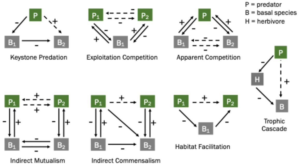
Density-mediated effects: when one species affects a second species through its impact on the abundance of a third species.

Trait-mediated effects: when one species affects a second species through its impact on the phenotype of a third species (e.g. changes in behaviour, habitat use, morphology).

Fisherman and seal compete for commercially valuable fish (hake). Fisherman thus removed seals to make it easier. Seals have direct negative effect on hake, but indirect positive effects on hake (seals eat their predators and competitors as well).

Trophic cascade: when rate of consumption at one trophic level results in a change of species abundance/consumption at lower trophic levels.

• Keystone species in intertidal zone change the game and their removal will affect many levels.

• Pisaster (keystone species) removal experiment

  • within months, barnacles dominated experimental plots. Then mussels took over. Algae disappeared and did most primary consumers. Sea star keeps barnacles and mussels in check, and their removal triggered a trophic cascade that impacted multiple trophic levels.

Trophic facilitation: when a consumer is indirectly helped by a positive interaction between its prey and another species. Juncus has an indirect effect on aphids in a salt marsh due to its impact on aphid food.

Competitive networks: interactions among multiple species that interact directly in negative ways (no one species dominates because of indirect effects)

Competitive hierarchies: one species dominates interactions (asymmetrical competition, amensalisms)

Dominant species: species that have a large effect on a community because it is more numerous or has the highest biomass within that community. Antelope, trees, ants.

Keystone species: species that affect other members of community in ways that are disproportionate to its abundance/biomass. Beavers, sea otters, and hippos

• Ecosystem engineers: species that are actively shaping their physical environment in ways that create habitat for other species. Beavers and hippos.

• Foundational species: species that provide structural habitat for others. Sea otters, trees, coral reefs, kelp, mangrove.

• Species do not always provide the same role in all communities where they are found - beavers in lakes that have been created by other means are not acting as keystone species. Deer are only dominant when apex predators do not control their numbers.

Metapopulations and Metacommunities

Species interactions affect community structure

There are two models of community organization:

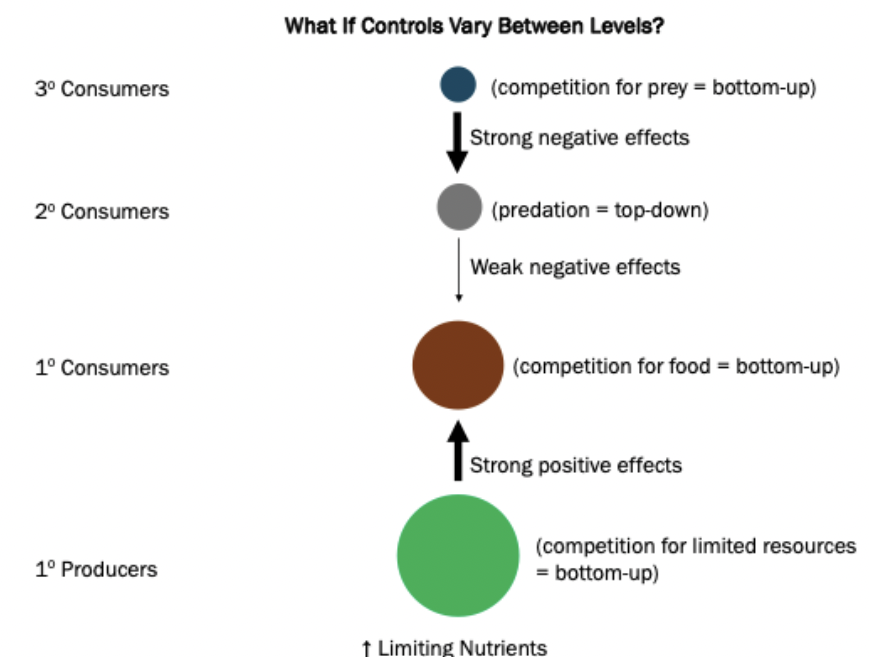
Bottom-up regulation: Nutrient availability at the bottom of the food chain controls the biomass at higher levels

Top-down regulation: Predation controls community organization (trophic cascade)

Both play a role. Predators control regulation. If everything is bottom up, it’s bottom up regulated. Species differ. It’s top-down or bottom-up when it’s dominated by one. Changes in nutrients trigger different things.

Controls may vary between levels. 2ndary consumers can have weak impact on primary consumers, but strong negative effects, so the strong negative outweighs making it top-down

Why is the world green? Autotrophs. It occurs by it’s own limiting food or predator. When wolves are remove, deers consume too many tree and this changes the green structure to a brown one. May lead to different symbiotic relationships. In absence of herbivory controls, plants should be dense and limited by competition.

The green world hypothesis: the world is green because herbivores do not control producer biomass. Most producer biomass moves through brown food web after producer dies. Consumers cannot do too much to plants because the things above it is stopping it from doing too much damage.

• Predictions: Food chains of given length increases in primary productivity, apex predator reduction will lead to alternating increases and decreases (trophic cascade), and an increase in potential productivity should lead to an increase in the number of trophic levels that can be supported by that ecosystem.

Metapopulations

Panmixia: Individuals freely move around habitat/range, also freely interbreed with other members of species → NO population structure, geneflow is widespread. Species that show panmixia are highly mobile. Good disperser, interbreeding habitat. Move, likely to find mate, not much structure, no genetic isolation, one giant population.

• Snail kite - patchy distribution, highly mobile and breed in ephemeral habitats.

Woodland species are more likely to breed with self than others. Dispersal is less and less likely with fragmented habitats. They exist in patches as suitable habitats. Can’t exist long term. Don’t stay in matrix very long. Higher risk predation. Different population linked by dispersal events. Matrix is a barrier. Dispersal is less frequent with the matrix.

Metapopulation: local populations can exist in patches of suitable habitat surrounded by areas of unsuitable habitat. Different populations connected by dispersal events. Patches can be recolonized by dispersal after populations have gone locally extinct.

• A population of subpopulations connected by gene flow / patchy environments

Levins (1970) → set of local subpopulations that persist in balance between random local extinctions and establishment of new local populations.

Dispersal can be individuals or just their gametes. Emigration and immigration between subpopulations is rare. Intervening habitat (called the habitat matrix is a barrier to dispersal.

Levins’ assumptions:

1. Patches identical and connected, discrete

2. Either occupied or empty, quickly reaches carrying capacity

3. Constant rate of extinction (m)

4. Patch colonization rate is proportional to the per patch colonization rate (c), multiplied by the fraction of patches currently occupied (p), multiplied by fraction of patches that are empty (1-p).

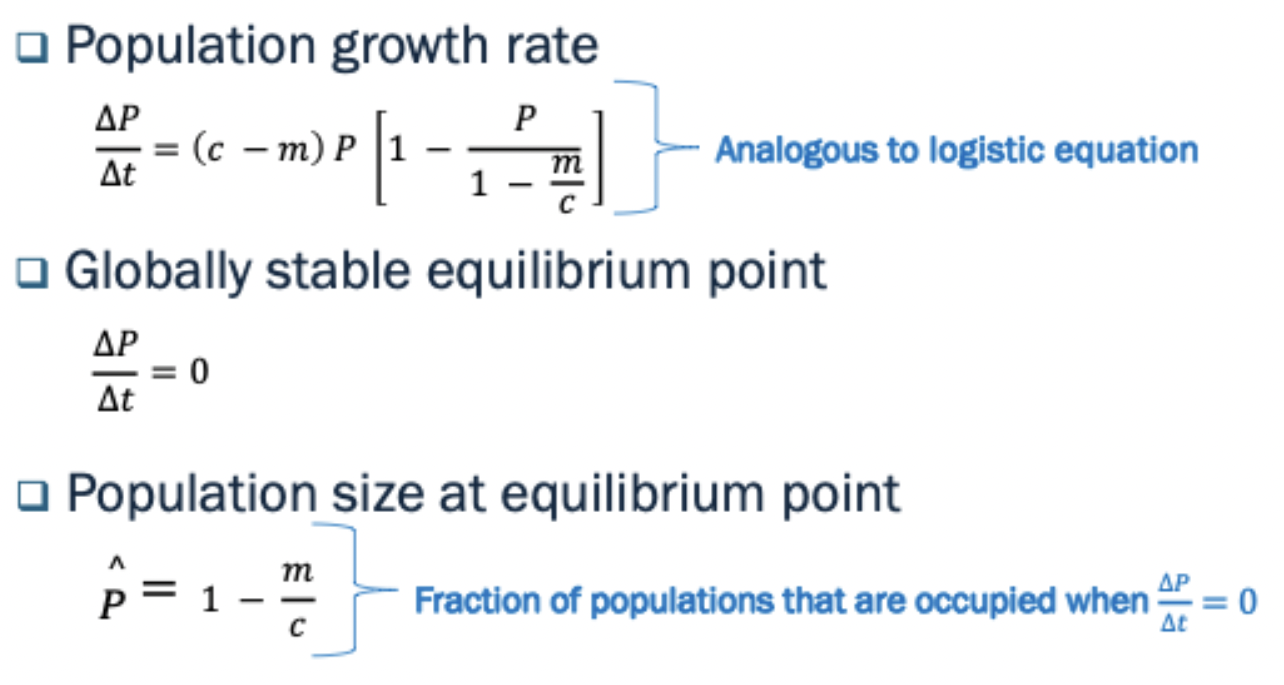
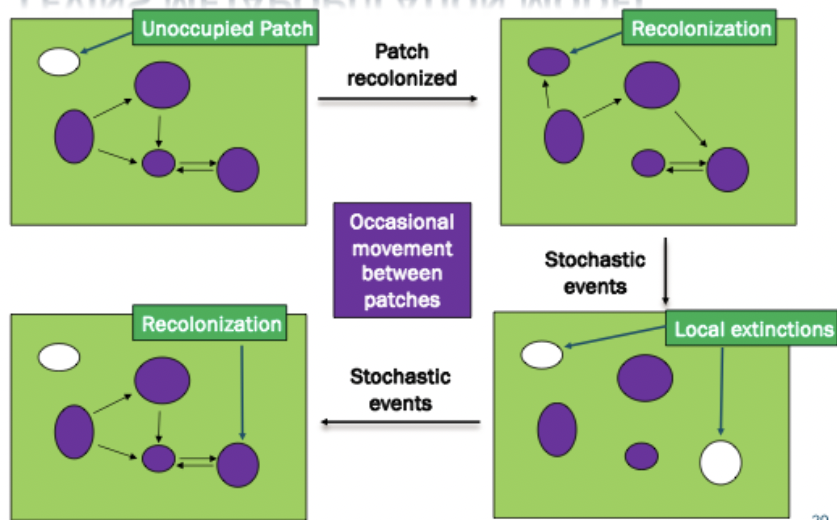
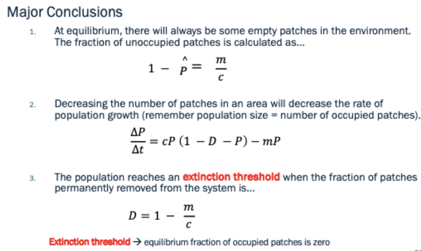
Empty habitat patches. If it is connected by dispersal events, empty habitat patches are in the role. You can cause stability of metapopulation based on what is added. Extinction threshold. You can model it. You can look at a bunch of different things to help make predictions.

Conditions necessary for stable metapopulations:

1. Suitable habitat and discrete patches

2. All populations have substantial risk of local extinction

3. Habitat patches must not be too isolate to prevent recolonization

4. Dynamics of local population are not synchronized.

Replacement of island biogeography theory. Helps predict future habitat and gauge situation.

Dispersal limitation: species is unable to occupy all suitable patches in its environment. This has some important consequences for population dynamics, species coexistence, community structure.

• Tropical bird species → Capture terrestial wrens. observed time took to return to home territory in presence and absence of corridors. Forest corridors can increase the movement of interior species between habitat patches - increasing species richness.

• Plant species richness → longleaf pine. difference of species richness of connected vs. isolated patches increased over time. patch corridor can aid in biodiversity.

Extinction debt: delayed extinction that occurs years after critical loss of habitat has occurred

• Breakdown of metapopulations because of habitat loss. Isolate populations.

• “living dead” - conserving current habitat will have virtually no effect.

Assisted dispersal (assisted colonization, migration): involves deliberate movement of species to new suitable area. Species moving risk not establishing, creating an invasive species. Species go and can be restored.

Metapopulation dynamics

Empirical models:

1. Classic metapopulations: Levins’ model, will all populations assumed to be similar in size and type. All populations at risk of extinction can also be recolonized afterwards.

2. Mainland-island metapopulations: Large population or patch acts as a mainland (lacks sig risk of ext), smaller populations are islands with more risk of extinction (source-sink dynamics)

3. Patchy populations: Individual within a single interbreeding population are clumped in space, but clumps do not exist as separate populations (high degree of gene flow) (panmixia?)

4. Nonequilibrium populations: Extinction is not balanced by recolonizations (goes and stays extinct). No gene flow to recolonize or rescue effect. Entire population will go extinct if all local populations disappear. Categorical, variation.

Sources: high reproductive success in good patches

Sinks: low reproductive success in poor patches.

Individuals move from source to sinks in a density dependent manner. Emigrants outnumber immigrants in sources. Sources keep sending over immigrants. Rescue effect is a big thing here.

Habitat loss:

• Habitat fragmentation: can create metapopulation structure. Patches shrink, become more isolated, it’s harder to recolonize. Extinction rate > colonization rate you get non-equilibrium.

• Isolation by distance: patches that are further apart are more isolated, reducing colonization rate. close too much gene flow, far not enough.

There are groups and distances where it becomes too far to colonize or 50% of population can no longer colonise.

Rescue effect: reduced when patches are further apart.

Case and Taper model:

• Interspecific competition, environment gradients, gene flow, and the coevolution of species borders forms a model. Species one and species two have a venn diagram of possible range. Edge populations aren’t happy compared to middle ones (sinks on the outside).

• Gene flow between populations is a source/sink dynamic. More individuals = more babies = more immigrants.

• Region of sympatry: sink with a competitor now. Fighting with yourself and others for resources. After secondary contact separates it from adaptive radiation.

  • Density compensation - greatly impact size of population in zome

  • Worse competitors may be competitively excluded, undergo character displacement (niche partitioning).

  • Competition and colonization trade-off - both persist.

Fugitive species: inferior competitor can exist because it is better at colonization (escaping, constantly on the move).

Opportunistic life history: individuals with high fecundity, grow quickly, reach sexual maturity at early age, produce many offspring (dandelion).

Alternating strategy.

Competition/colonization trade-off: two or more competitive species can coexist in a patchy environment when there is a trade-off between competitive ability and dispersal ability

• If both have equal mortality rates (m), then both species can persist in area only if inferior competitor has the superior dispersal ability.

• C2 > C1m → the C’s stand for colonization rate

• Species compete in competitive hierarchy, the better competitor competitively excludes other from any patch it is in, there is a strict tradeoff between the ability to compete within a patch, and the ability to colonize a patch

  • How species coexist ^

Seed size / seed number trade off → many small is little to no parental investment, few large offspring has high parental investment.

• Mortality risk

  • High mortality risk at all age levels: invest into each offspring and have a lot, to increase the chances that at least some make it

  • High juvenile low adult mortality: put more into each offspring so when they become large adults sooner.

  • Ratio of adult to juvenile mortality determines packaging of reproduction. If you’re safer as an adult, they’ll make you real big real quick.

• Competition

  • resources unlimited: invest little into each offspring and have a lot because offspring are capable of finding their own resources

  • Resource limited: have a few, large offspring and invest in parental care.

• Real world is very complex and other mechanisms can also explain occurences of coexistence of competing species.

• Species can coexist through a dispersal / fecundity trade-off

  • more fecund species are more successful when patches are close together and better disperser species are more successful when patches are further apart.

When landscapes are heterogeneous - other ways of coexistence becomes possible. Like niche partitioning, and colonization related tradeoffs.

Eusocial ants are established by one or two queens. When they die, so does the colony. Dispersal of future queens decides everything. There is a happy coexistence for ants of positive fecundity and positive dispersion - somewhere in the middle.

Tolerance / Fecundity Tradeoff: consider an environment containing multiple patch types (patch heterogeneity). Species can now differ in tolerance of different patch types. Species can differ in possibility of reaching a patch.

Difference in colonization ability: modifies conditions needed for coexistence, has impact on relative species abundances in different patches

Metacommunities

Local community: all the species that potentially interact with one another in a single locality

Metacommunity: set of local communities linked by dispersal of one or more of their constituent species. Tying different regions together. Impact in metapopulations.

Patch dynamics: extension of metapopulation model to more than two species

Mass effects: extension of principles of source-sink dynamics and rescue effects to multiple species. Change in alpha/beta.

Species-sorting: emphasizes differences in species’ abilities to utilize different patch types in an heterogeneous environment. What if dispersal is perfect for people picking an area and staying.

Neutral: assumes species are functionally identical and that niche differences are unimportant

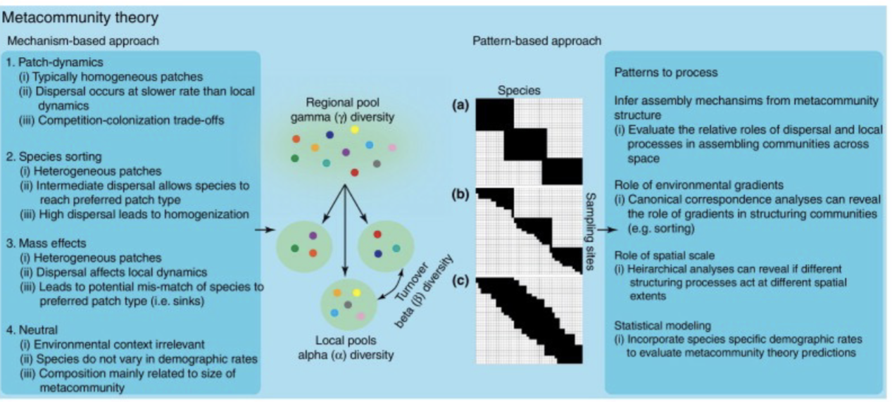
Dispersal of individuals from source to sinks can have significant effects on population dynamics and species diversity within local community. Rate of movement between local communities can affect diversity at multiple spatial scales.

Three assumptions model:

1. Each local community contains S species that are competing for limited vacant patch

2. Metacommunity consists of N local communities (heterogeneous)

3. Constant proportion (a) of each local population disperses between communities.

No dispersal: each local community dominated by best local competitor. alpha diversity low and beta and gamma at maximum.

As dispersal increases: alpha increases, beta decreases, gamma remains the same.

As dispersal exceeds threshold: a decrease, beta slight rise, gamma decline.

At high levels of dispersal: metacommunity functioning as one large community, best regional competitor exclude other species entirely. All levels of diversity are at their lowest as a result.

Mass effects perspective: invertebrate diversity varies with pool isolation. Intermediate pool isolation has alpha really high. Higher dispersal potential showed no relationship between species richness and isolation distance. Passive dispersers are boring basically.

Metacommunities and Variable Environments

Patch dynamics: extension of metapopulation model more than two species in a homogeneous environment

1. Environment is composed of homogeneous patches separated by inhospitable matrix.

2. Dispersal very low - slower rate than local dynamics

3. Competition colonization tradeoff exists.

Species-sorting: species differ in their ability to utilize different patch types in a heterogeneous environment.

1. Dispersal occurs at relatively low rate (movement of individuals between local communities does not have a direct effect on population abundance within a patch, or affect the outcome of species interaction within a local community. → no mass effect)

2. Dispersal rate is sufficient for all species to reach every locality where they can persist. Conclusions: environmental variation predicts species distribution. Dispersal is solo. Species from regional pool figure it out.

When you vary in dispersal rates, enough to manage source-sink dynamics, you have mass effects (maintaining weaker competitors/rescue effect). Species sorting shows just enough effects. With climate change, they’re going to need to be able to do that.

Regional pool - colonize tidal zones. Determines local community and how to handle climate change. Things shift and species die. No dispersal → just enough dispersal to stay alive. Species sorting effects are just robust enough for climate change.

Marine system and local freshwater are different. If you’re maintaining a regional pool, they are also doing that. If you can have a regional pool and can maintain, help maintain diversity - you are less likely to lose biodiversity. Even a little diversity can have crazy effects.

Neutral perspective: all species are functionally equivalent (lack of niche, lack of species differences), and have identical per capita birth, mortality, and dispersal rates.

Assumptions:

1. Number of individuals in community is constant. Space is limiting and all space is occupied. If one species enter, abundances of other species decline to make room

2. All individuals, regardless of species, have equal probability of colonizing open space.

3. Death occurs at a constant and fixed rate.

Very slow - time they take over, by the time they take over, they could be two species. Speciation outpaces local extinction.

Spatial turnover in forests is greater than the neutral theory predicts. Also in temperate forests → model was not a good fit for observable patterns

Rocky intertidal zone showed mixed support for the neutral theory → good fit for general shape of species abundance, but not species dynamics over 7-11 year time frame.

Neutral model is a good null model, real world communities exist on a continuum of niche and neutral interactions. The focus of the model is on dispersal and regional species pool interactions ← metacommunity perspective.

Mechanisms of coexistence

Stable coexistence: species tend to recover from low densities and species densities do not show long term trends. Species abundances vary, but all species persist in area.

Stable equilibrium is rare, showing growth while the other reaches their own carrying capacity. Positive growth, when there’s not many of you and you’re struggling. You’re your own worst enemy.

Unstable coexistence: species may coexist within a community for long periods as a result of slow rates of competitive exclusion. No mechanism promoting species recovery. Neutral theory assumes unstable species coexistence (inter and intraspecific competition). Long term diversity maintained through immigrants.

• Any changes in population size due to any disturbances will cause one species or the other to go to fixation (to increase towards its K, competitively excluding the other species over time).

Equalizing mechanisms:

• Make you equal, neutral approach is relevant here

• On a spectrum, the closer the competitive ability, closer to equalizing/neutral approach. More likely one will be faster.

• Overtime biodiversity goes down, tend to show up in system with regular disturbance

• Intertidal zone and fighting for space: better competitor shows up and stays there until wave comes around and resets.

Stabilizing mechanisms: Favour species recovery when it becomes rare. Reduced fitness difference between them. When you’re common, you’re the target.

• Resource partitioning, other niche-based mechanisms that increase the strength of intraspecific competition wrt to interspecific competition

• Fluctuation-independent mechanisms: operate whether the environment fluctuates, or it doesn’t

• Fluctuation-dependent mechanisms: require fluctuations in population densities and environmental factors to operate.

  • Relative nonlinearity of competition: two or more species can coexist on a single, limiting resource if their functional responses have non-linearity. Resource abundance needs to fluctuate.

    • Some species are favoured when the resource abundances are low. If resources are interchanging their popularity, different resources are relevant at different time. Fluctuations favour different competitors and create stable coexistence.

    • When ABIOTIC resources fluctuate: Lower R*, both bring it down till eventually YOU win competition. If/when resources fluctuate - at resource level vary over time, sometimes you're making so many babies you're replacing yourself or you're just eating to survive idk. More babies when low population.

    • If resource is a limiting thing, stable climate limit cycle. Interaction between biotic resources and their predator can generate temporal variations.

    • When BIOTIC resources fluctuate: differ in FR of nonlinearity to survive. Neither predator can dominate. Asynchronous fluctuations in abundances of different predator species.

    • Two or more consumer species can coexist on a single, limiting resource if their functional responses have nonlinearities. (type 2, type 3)

  • Storage effects: species store effects of good years as a buffer against the impacts of bad years. Storing seeds.

    • Lottery model: early model of storage effect, named for the way competition for space was determined. Studying competition of reefs and fishes. Many never find territory. Many babies, few get a territory. Once you get it, it's yours for life. As long as adults are there they can wait and wait. No one species can win - equal chance of getting it, so rare for them to empty. Adults carry on for life.

      • Iteroparous / overlapping generations

      • Larval fish need to obtain territory. Always more larvae than territory.

      • Abundance of larvae

      • Larval survival depends on environment.

    • Adults are long-lived and store effects. Adults buffer species against effects of bad years because adults hold onto their territories for life.

    • Pine trees survive around hardwood because they vary temporally, waiting for forest fires.

      • Species specific environmental response (so not every species always has a good year)

      • Buffered population growth (exist as seeds over time).

      • Covariance between environment and competition. Bad environment decrease competition, good environment increase competition.

Variable Environments and Agents of Change

More microhabitats (spatial heterogeneity) → more biodiverse

Environmental heterogeneity x species richness → correlation

• different areas in a river have different animals

Environmental harshness: extreme habitats typically dominated by an extreme abiotic factor. Special morphologies in species. Low plant productivity. Hard to prove lower species richness in harsh environment.

Intermediate disturbance hypothesis: frequent disturbance favour good colonizers, rare favours good competitors, and intermediate neither is favoured.

Pioneer species: early colonizers that persist in a community based on their ability to colonize/recolonize after disturbances (opportunistic species)

Climax community: final stage of succession, mature assembly of best competitors (equilibrial species) that persist until a disturbance leads to local extinction.

Succession has trajectory. Oak hickory climax. Series of competitivie exclusions cause successional changes.

Facilitation → early successional species modify physical environment in ways that favour invasion by later successional species. Soil and shade.

Primary succession is no life - the minute you get even a root it is secondary succession. Plants need help entering a sand dune. Waves.

Inhibition: early arrivals inhibit invasion of later species, but cannot completely prevent their appearance ← slows succession down, but does not stop it. Common around water, later become established through disturbance.

Algal succession via inhibition.

Faster dispersal: early successional species are better colonizer, later are better competitor

Relative growth rates: early and late successional species all arrive together but early species grow to maturity faster.

Tolerance drives succession.

Our soils are not very deep, glacial action. Glacial retreated, volcanic eruptions, emergence of new islands.

Volcanic eruption succession: we want to free-up potassium. Rock needs to be weathered, lichen moss community dies, builds up soil layer with decomposers.

Secondary succession: recolonization following a disturbance the only partially removed species from area. Some species persist as either adults or in a seedbank. One tree falls, or wildfire wipes them all out.

Following fire: Soil can kill off decomposers in forest fires, too hot.

There are abiotic agents of change (stress or disturbance) or biotic agents of change (competition, predation, trampling, digging).

Intermediate disturbance hypothesis → in dominance-controlled communities, gaps that are created by disturbance will then undergo through succession. May be visible on an incline.

• Successional mosaic model: High levels of biodiversity when it resets. Explains clearings, edging (species didn’t leave, they just jumped around the forest), storage effects (exist as seeds and wait for fire to free things up).

  • Disturbance resets succession within a patch because it opens space. Species coexistence because there is a system of patches at different successional stages.

  • Assumes competition/colonization trade-off

  • Habitat heterogeneity favours competition / colonization trade-off. This differs from other models based on this tradeoff, which require homogeneity of patches.

You can get absolutely brutal fires or none at all.

Wave action can control succession - highest on small boulders, lowest on large ones. Green algae first to recolonize, then series of successional changes occur. Small rocks dominated by green algae. Large boulders dominated by G. canaliculata. Strongest competitors get favoured with minimal disturbance. Remove top down is bad - monoculture of best competitors.

Disturbance fixes everything. Mowing above ground vegetation is an act of defiance. Human actions lead to something in alternative states. Regime shift.

Alternative stable state: sometimes different communities develop in same area under similar conditions. Human actions can lead to switch alternate state (Eg. coral reef → algal communities)

Regime shift (phase shift): a change from one community state into another state

Tipping point: a critical threshold that, once reached, will trigger a regime shift in a system

Resistance: the strength of a perturbation needed to cause a regime shift in a system

Resilience: the speed at which a community recovers from a perturbation

• Ecological resilience: largest magnitude of perturbation that a system can handle without undergoing a regime shift

• Engineering resilience: the time it takes a system to recover from a perturbation

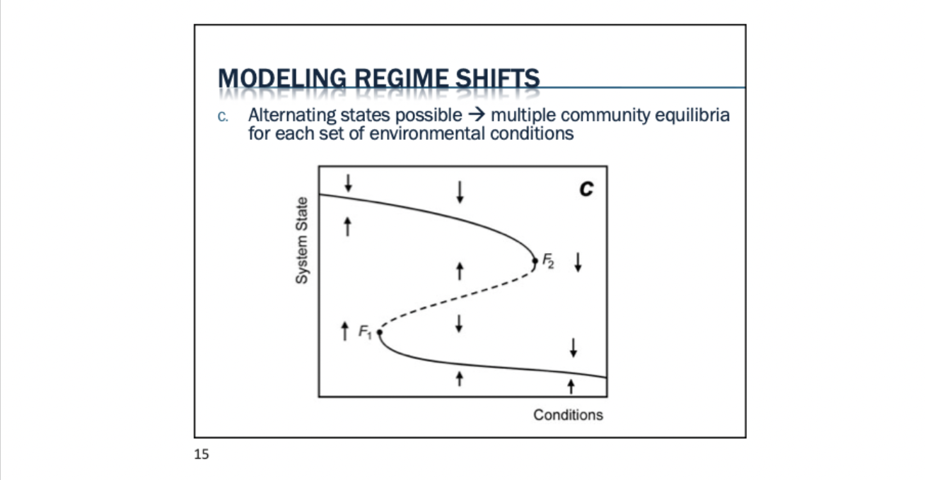
Same set of conditions can create different communities. Founder control communities. Far rarer. Didn’t think it existed in classical conditions. One factor triggers change, everything exactly the same. Typically called alternative state.

With alternative stable states - communities with different configuration that represent alternate equilibrium states (alternate ‘climax communities’ under similar environmental conditions). Communities might differ in species richness, composition, food web structure, size structure, etc.

Hysteresis: delayed response to forward and backward changes in environmental conditions (e.g. need to reach a tipping point before can change to alternate community).

There was a regime shift with coral bleaching - There was warmer water. Changes in the South Pacific Ocean changed everything (el nino event). More minor component. Took over the reef, surviving disturbances and recovering. Second type of coral was dying off. Belize was trying to regrow the reefs - requires a lot, and they’re still at risk with the temperature issue. Staghorn coral was wiped out due to warm and disease. Then a regime shift (el nino event) wiped out the second coral.

Premier beaches are susceptible to erosion due to wave action/storm surges ← coral reefs protect beaches from this erosion. Severe reef damage has occured due to overfishing, sedimentation, water pollution. rising sea level, more erosion. Reefs can rebuild after disturbance, but need time. Brazil protects blue parrot fish which eat algae and give coral time to rebuild.

Regime shifts in the ocean: species of anchovy and sardine differ during different periods. 3D printing coral. Predictable changes in 7 year cycles (el nino, la nina). Decomposition (upwelling) - pulling up nutrient rich water to the surface is causing regime shifts.

With temperatures increasing, we see a lot more regime shifts. No fish living. If things can’t adapt to heating up, we might end up with nothing there. Issue with equator being the most biodiverse - might no longer be so diverse.

Evolutionary Community Ecology

Co-evolution: development of genetically determined traits in two species to facilitate and interaction. Species interactions that lead to co-evolution often mutualistic/beneficial → coevolutionary arm’s race

Symbiotic mutualism can lead to coevolution. Can be antagonistic as well. Predator/prey - prey evolving to escape while predator evolves to be better at catching prey.

Predators:

• Pincers used to handle prey

• Forward facing eyes are predatory (see depth, can’t see behind though) while prey to see 360.

• Toxins

• Aggressive mimicry (make approach more subtle)

• Dragonfly best brain at predicting where fly will end up

• Whales and dolphins good at faking traps. Create bubbles and just wait there.

Preys:

• Hiding in plain sight

• Lie, startle them and have time to escape.

• Unappetizing, cryptic and aggressive mimic.

• I can defend myself, go find another deer

• Hawk faster than rabbit, but rabbit turns quicker

• Bright colour = I taste bad

• Mimic something that does taste bad.

Sexual conflict: one biological sex evolves to be ‘more charming’ other sex evolves to find traits less charming. Other biological sex trying to be discerning.

Sexual selection arm’s race: increase duration of sec, females can be better at evading. Hooks, deter hooks. Scrubbing sperm out, copulatory plug. So many arms races in insects. Tail, females like tails, close relatives don’t have tails.

Extreme forms show up in arm’s races.

Plants will deter herbivory. Competition play role. Might grow more root biomass instead. Everything affects your fitness.

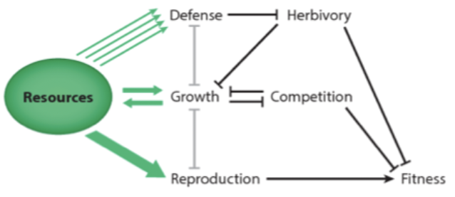
Defense-competition trade-off: the costs of predator defense can lead to a trade-off with competitive ability if it impacts individual fitness

Narrow genotypic variation: fixation of the best predator defense trait in prey over time (loss of genetic variation, thus loss of competitive ability)

Wide genotypic variation: oscillations in prey and predator densities → prey defensive trait variation maintained due to temporal variation in direction of selection and rate of evolution (alternating between selection for defensive ability versus selection for competitive ability over time → balancing selection for both).

Fluctuating selection: changes in direction of selection on a given phenotype over time results in both alleles being maintained

Algae help us learn how multicellularity developed. They formed colonies. Ability to form colonies is a heritable trait, but it comes at a cost of decreased competitive ability, resulting in reduced population growth.

Narrow genotypic prey defense variation: Within one predator-prey oscillation, prey evolved to fixation on one moderately well-defended genotype, and predator + prey populations were in equilibrium.

Wide genotypic prey defense variation: Dominant algal genotypes alternating over time between well defended colonies and vulnerable small colonies / single cells.

Community Ecology in Action: Restoring Ecosystems

Ecological resilience - natural ability of an ecosystem to recover from a disturbance

• Humans can do a lot of damage. Not even touching, but chemical pollution can affect things from separate areas. Flooding - we’re bad at cleaning up our waste. Without human intervention - many degraded ecosystems can take centuries, or even longer, to recover. Others may never recover at all.

Ecological restoration: practice of restoring species/ecosystems in an area to a point in time before they were degraded, damaged, or destroyed (theory)

Restoration ecology: science of ecological restoration, research, scientific study of restored populations, communities, and ecosystems. (practice)

One is the theory and one is the practice that tests the theory.

Do restoration ecology by coming up with a plan, site specific plan. Adaptive management: need to be able to change, might be a cycle. If restoration is not working, change the ecosystem you’re in.

Most of Ontario’s forest were deforested to build boats, and their forests are now secondary growth. Forest were able to regenerate.

Four main approaches:

1. No action (passive restoration): recovery possible without human intervention, or restoration has previously failed or is deemed too expensive.

2. Rehabilitation: degraded ecosystem is replaced with a different, productive one (can involve replacement of a few species, or many species).

3. Partial restoration: at least some of original ecosytsem functions/species are restored (typically, focus is on dominant species, resilient species, keystone species, leaving rare species for later).

4. Complete restoration: original ecosystem, complete with species composition/community structure, restored through adaptive restoration, after original cause(s) of loss are mitigated.

If we have to keep intervening - money might be better spent elsewhere. Lots of non-scientists get involved. Take into account local knowledge.

Factors that will contribute to decision:

• Speed of restoration, cost involved, reliability of results, ability of target community to persist with little to no future maintenance

Restoration projects will therefore be multidisciplinary, involving people with both theoretical and application knowledge

Practical consideration

What type of action is required to restore ecosystem?

• Most degraded may require both physical and biological alterations. If the damage was caused by a specific abiotic factor (e.g. water overdrafting) will need to address original cause first

• Can’t just return species, you may have to do a bunch of soil and rocks. That’s physical alterations. Stop water alterations - remove the stressor.

• Restoring ecosystem function: Adjusted management. More degraded, nonfunctional sites likely have abiotic constraints contributing to the problem. Biotic barriers require planting, reintroducing missing trophic levels, providing prey as food source. Mostly intact ecosystems may only need better management strategies.

Ecological assembly order

• What order should species be restored? When should they be restored?

• Trophic-level decisions are easier, because prey populations must be established before predators are reintroduced. Overlaps in functional relationships make decisions harder → if they have multiple species with similar ecological role, what order should we use?

• Niche overlap is bad. Niche complementarity is good. Plant functional type is important.

Genotypes of species that are being reintroduced

• Local-is-best (LIB) approach: prioritize locally adapted genotypes, where possible - local adaptations impact likelihood of species persistence in area. Reduced risk of outbreeding depression within area. Reduces chances of genetic swamping from nonlocal genotypes.

  • Too much interbreeding may need to start going out

  • Heavy helmet peregrine falcon - city ones don’t do well with northern ones. Local genetic in northern were lost.

• When LIB is not feasible: may rely on more distant populations → too small or could be harmed

Gaining support / participation of local stakeholders

• Restoration efforts often initiated by local conservation groups are recognized between environmental health local people’s economic and personal well being

• Can also receive funding from local landowners, conservation groups, or other support by those who manage the area

Adaptive Restoration

Involves active management of area post-restoration, costly, requirement to ensure long-term success of restoration

Passive restoration is when ecosystem recovers naturally.

When we do it actively:

• Native species that failed to thrive may need to be supplemented, ones that failed to survive may need to be reintroducing natives

• Secondary invasion: a different invasive species has entered area and needs to be removed

• Removing roads/other human infrastructure, restoring connectivity, repairing soil, etc.

Restoration ecology to date: efforts to restore degraded terrestrial communities have focused on re-establishing original plant community. Growing recognition that we can’t ignore the other major components of the community (fungi/bacteria, herbivore mediated-coexistence, birds and insects, and birds and mammals → pollination and insect population control, seed dispersal, and soil digging).

Novel ecosystems: may not be possible to restore original ecosystem if human activities have too greatly altered environment. Contain a mix of native and exotics may be the best we can do. Not perfectly the same.

Reconciliation ecology: development of urban places where people and biodiversity can coexist.

• Goal: to find ways to promote and protect biodiversity in human-dominated landscape

• Potential habitats: landfills, city parks, green roofs, privately owned backyards, golf course (ponds or fringe habitats)

Fresh kills landfill (Staten Island) → Became biggest park. Barrier between garbage and land. Garbage decomposes to methan. Good, saved New Jersey millions of dollars while flooding.

Pollinator corridors - provide critical grassland habitat - mowed lawn between grassland habitat for many species

Similar habitats are created by mown powerline fields → especially for infrequently mown areas that are not treated with pesticides

Green roods and city parks can create habitat within human-dominated landscapes. Resist to changing temperature. Rouge landfill. Restoration ecology in park.