L3_Computer Vision and the concept of layers

Shallow Learning vs. Deep Learning

Shallow Learning

• Employs engineered features derived from original features, often requiring domain expertise for effective feature crafting.

• Limited in their ability to learn complex patterns directly from raw data.

• Model: y = f(x1, x2, x3, x4,…, x_n|\theta)

Deep Learning

• Learns feature representations sequentially through multiple layers of neural networks, enabling automatic feature extraction from raw data.

• Excels in handling high-dimensional data and capturing intricate relationships without explicit feature engineering.

• Model: y = f3(f2(f1(x1, x2|\theta1)|\theta2)|\theta3)

• Key idea: Sequentially learn hierarchical feature representations, where each layer refines the features learned by the previous layers to solve complex tasks.

• Neural networks are universal function approximators, capable of modeling highly complex and non-linear relationships, making them suitable for a wide range of tasks.

• Requires a significant amount of data to effectively train the numerous parameters and avoid overfitting, especially due to the model's complexity.

Feed-Forward Neural Network

• Each node computes an output by applying an activation function to a weighted sum of its inputs plus a bias term. The formula is: y = f(\sum{i=1}^{n} wi x_i + b)

  • w_i: Represents the weight of each incoming connection, determining the strength of the connection.

  • b: Represents the bias term, which allows the neuron to activate even when all inputs are zero, adding flexibility to the model.

  • f: Represents the activation function, which introduces non-linearity to the model, enabling it to learn complex patterns.

    

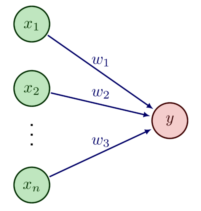
Image Classification

• The goal is to accurately classify an image into one of several predefined categories based on its visual content.

• Naive approach: Treat every pixel as an individual feature and feed these features directly into a classifier.

Issues with Pixel-Based Approach

• Not invariant under translation: Shifting the image even slightly can drastically change the pixel values, leading to incorrect classifications.

• Not invariant under dilation: Resizing the image alters the pixel arrangement, causing the classifier to misinterpret the image content.

Convolution Operation

• Acts as the cornerstone of modern computer vision by enabling the detection of patterns regardless of their position in the image.

• Takes two functions as input and produces a new function that expresses how the shape of one modifies the other: f * g \equiv \int_{-\infty}^{\infty} f(\tau)g(t - \tau)d\tau

• In practice, convolution is used to recognize and localize patterns in images and other data by sliding a kernel over the input and computing the dot product.

Discrete Convolution

• Adapted for processing discrete data, such as images represented as arrays of pixel values.

• The integral is replaced with a summation, making it computationally feasible for digital image processing.

• The first function typically represents the input image, providing the data to be analyzed.

• The second function is the kernel, a small matrix of weights used to detect specific features or patterns in the image.

Convolution over Images

• Simple Case: One input channel, where the kernel slides over the single-channel image to produce a feature map.

• RGB Color Images: Each color channel (Red, Green, Blue) is processed independently with the same or different kernels, and the results are summed to produce the final feature map.

Convolution Kernel (or Filter)

• Convolution with carefully designed kernels forms the basis of digital image processing, allowing for various image manipulations and feature extractions.

• Applications:

  • Identify vertical lines by using kernels that respond strongly to vertical edges.

  • Identify diagonal lines through kernels designed to detect diagonal patterns.

  • Identify horizontal lines with kernels sensitive to horizontal edges.

More Filters

• Average Filter: Creates a blurring effect by averaging the pixel values in the neighborhood. \frac{1}{9} \begin{bmatrix} 1 & 1 & 1 \ 1 & 1 & 1 \ 1 & 1 & 1 \end{bmatrix}

• Sobel Filter: An edge detector that highlights edges by measuring the rate of change of the image intensity. \begin{bmatrix} -1 & 0 & 1 \ -2 & 0 & 2 \ -1 & 0 & 1 \end{bmatrix}

Kernels for Image Recognition

• Handcrafting filters/kernels requires deep domain knowledge and can be a tedious process.

• Refining this approach involves learning the kernels directly from the data.

Decomposition into Simple Patterns

• A more effective approach involves using multiple small filters to capture different aspects of the image.

• Process:

  • Start with the original image.

  • Generate a new image at a lower resolution to reduce computational complexity.

  • Repeat the process iteratively, extracting increasingly complex features.

• Example: Breaking down an image of a cat into simpler patterns, such as edges, textures, and shapes.

Keras Layers

• Convolution layers: Extract intricate image features by convolving the input with a set of learnable filters (keras.layers.Conv2D).

• Pooling layers: Downsample the feature maps and aggregate the features, reducing spatial dimensions and computational load (keras.layers.MaxPooling2D).

• Fully-connected (dense) layers: Compute the final classification or prediction based on the high-level features extracted by the convolutional and pooling layers (keras.layers.Dense).

The Conv2D Layer

• keras.layers.Conv2D

  • filters: Specifies the number of filters to learn, determining the number of feature maps to output (typical range: 32 to 512).

  • kernel_size: Defines the spatial dimensions of the filter, controlling the receptive field of the convolution operation (typical: 3x3, sometimes larger in the initial layer).

  • strides: Sets the step size for sliding the filter across the input, affecting the spatial resolution of the output feature maps (typical: 1 or 2).

  • padding: Manages the spatial dimensions by adding padding around the image edges.

    • "valid": Implies no padding, which may reduce the spatial size of the output.

    • "same": Applies padding to maintain the same spatial dimensions as the input.

Pooling Layers

• Reasons for downsampling image features:

  • Learn a spatial hierarchy by expanding the receptive field, enabling the network to capture more global patterns.

  • Reduce the total number of parameters, mitigating overfitting and computational costs.

• Most common approach: Choose the maximum value from a window of pixels, preserving the most salient features while discarding less important information.

The MaxPooling2D Layer

• keras.layers.MaxPooling2D

  • pool_size: Indicates the size of the pooling window, defining the spatial extent over which the maximum value is computed (typical: 2x2 or 3x3).

  • strides: Determines the step size for the pooling operation, often set to the same value as pool_size to create non-overlapping regions.

  • padding: Adds padding around the edges of the input to control the spatial dimensions of the output (valid or same).

The Dense Layer

• keras.layers.Dense

  • units: Specifies the number of nodes in this layer, defining the dimensionality of the output space. In the last dense layer, units must be equal to the number of classes (or desired outputs) to perform classification.

My First Convolutional Network

• Constructing a convnet using Keras' sequential model API.

• Example:

convnet = keras.Sequential(
    [
        keras.Input(shape=(28, 28, 1)),
        keras.layers.Conv2D(32, kernel_size=(3, 3), activation="relu"),
        keras.layers.MaxPooling2D(pool_size=(2, 2)),
        keras.layers.Conv2D(32, kernel_size=(3, 3), activation="relu"),
        keras.layers.MaxPooling2D(pool_size=(2, 2)),
        keras.layers.Flatten(),
        keras.layers.Dense(10, activation="softmax"),
    ]
)

• Model Summary:

Model: "sequential_1"
_________________________________________________________________
Layer (type) Output Shape Param #
=================================================================
conv2d (Conv2D) (None, 26, 26, 32) 320
_________________________________________________________________
max_pooling2d (MaxPooling2D) (None, 13, 13, 32) 0
_________________________________________________________________
conv2d_1 (Conv2D) (None, 11, 11, 32) 9,248
_________________________________________________________________
max_pooling2d_1 (MaxPooling2D) (None, 5, 5, 32) 0
_________________________________________________________________
flatten_1 (Flatten) (None, 800) 0
_________________________________________________________________
dropout (Dropout) (None, 800) 0
_________________________________________________________________
dense_3 (Dense) (None, 10) 8,010
=================================================================
Total params: 17,578 (68.66 KB)
Trainable params: 17,578 (68.66 KB)
Non-trainable params: 0 (0.00 B)

• Configure the training objective and strategy.

convnet.compile(
    loss="categorical_crossentropy",
    optimizer="adam",
    metrics=["accuracy"]
)

convnet.fit(
    X_train,
    y_train,
    batch_size=128,
    epochs=15,
    validation_split=0.1
)

Decomposition into Simple Patterns: Theory vs. Practice

• Classifying pictures of cats involves learning hierarchical features that capture different aspects of the image, from edges to textures to shapes.

Layer Activations

• Visualizing what each filter detects by examining its activation on a test image, providing insights into the learned feature representations.

• The output after the convolution operation and the application of the activation function reveals which features the filter is most sensitive to.

• Examples: Layer 1, filter 4; Layer 1, filter 7 display the activation maps for two different filters in the first layer.

• Repeat this process for all filters in all layers to gain a comprehensive understanding of the network's feature extraction process.