6.1 Bivariate Correlations

Bivariate Correlation: when we are considering the relationship between two variables

• If the two variables are associated, they are said to be co-related (correlated). This means they co-vary; as the scores on one variable change, scores on the other variable change in a predictable way. This means that the two variables are not independent.

6.1.1 Drawing Conclusions from Correlational Analysis

• A correlational relationship cannot automatically be regarded as implying causation. That is, if a significant association exists between the two variables, this does not mean that x causes y, or alternatively, that y causes x.

• Let us assume that the two variables, x and y, are correlated. This could be because:

  • the variation in scores on y have been caused by the variation in scores on x (i.e., x has caused y)

  • the variation in scores on x have been caused by the variation in scores on y (i.e., y has caused x)

  • the correlation between x and y can be explained by the influence of a third variable, z (or even by several variables)

  • the correlation between them is purely chance.

• Francis Galton invented correlation but Karl Pearson developed it, discovering spurious correlations (a statistical relationship only -- not due to a real relationship between the two variables).

• The exploration of relationships between variables may include the following steps:

1. Inspection of scattergrams.

2. A statistical test called Pearson’s r, which shows us the magnitude and degree of the relationship, and the likelihood of such a relationship occurring by sampling error, given the truth of the null hypothesis.

3. Confidence limits around the test statistic r, where appropriate.

4. Interpretation of the results.

6.1.2 Purpose of Correlational Analysis

• The purpose of performing a correlational analysis is to discover whether there is a meaningful relationship between variables, which is unlikely to have occurred by sampling error (assuming the null hypothesis to be true), and unlikely to be spurious.

• Correlational analysis enables us to determine the following:

  • the direction of the relationship -- whether it is positive, negative, or zero.

  • the strength or magnitude of the relationship between the two variables -- the test statistic, called the correlation coefficient, varies form 0 (no relationship between the variables) to 1 (perfect relationship between the variables).

6.1.3 Direction of the Relationship

Positive

• High scores on one variable (which we call x) tend to be associated with high scores on the other variable (which we call y); conversely, low scores on variable x tend to be associated with low scores on variable y.

Negative

• High scores on one variable are associated with low scores on the other variable.

Zero

• Zero relationships are where there is no linear (straight-line) relationship between the two variables.

6.1.4 Perfect Positive Relationships

Perfect Positive Relationship: where all the points on the scattergram would fall on a straight line.

5.1.4 Imperfect Positive Relationships

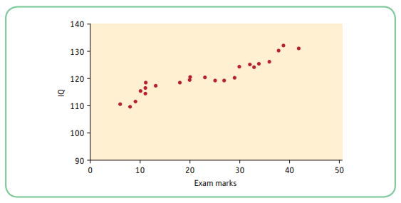
• For example, we want to see whether there is a relationship between IQ and exam marks. Based on the scattergram, high IQs tend to be associated with high exam scores and low IQs tend to be associated with low exam scores. In this instance, the correlation is not perfect but the trend is there, and that is what is important.

• Although the dots do not fall on a straight line, this is still a positive linear relationship because they form a discernible pattern going from the bottom left-hand corner to the top right-hand corner.

6.1.6 Perfect Negative Relationships

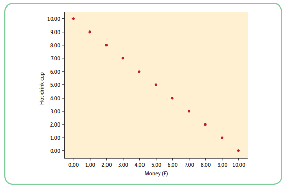
• Because this relationship is perfect, the points on the scattergram would fall on a straight line. Each time x increases by a certain amount, y decreases by a certain, constant, amount.

6.1.7 Imperfect Negative Relationships

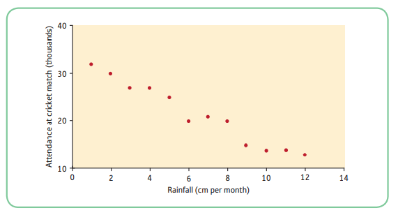
• With an imperfect negative linear relationships the dots do not fall on a straight line, but they still form a discernible pattern going from the top left-hand corner down to the bottom right-hand corner.

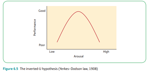
6.1.8 Non-linear Relationships

• If a relationship is not statistically significant, it may not be appropriate to infer that there is no relationship between the two variables. This is because a correlational analysis tests to see whether there is a linear relationship.

• Some relationships are not linear.

  • Example: relationship between arousal and performance. Although we would expect a certain level of arousal to improve sports performance, too much arousal could lead to a detriment in performance. This law predicts an inverted curvilinear relationship between arousal and performance. At low levels of arousal, performance will be lower than if arousal was a bit higher. There is an ‘optimum’ level of arousal, at which performance will be highest. Beyond that, arousal actually decreases performance.

6.1.9 The Strength or Magnitude of the Relationship

• The strength of a linear relationship between the two variables is measured by a statistic called the correlation coefficient, also known as r, which varies from 0 to -1, and from 0 to +1.

• Several Types of Correlational Test:

  • Pearson’s r

    • full name: Pearson’s product moment correlation

    • this is a parametric test

  • Spearman’s rho

    • a non-parametric equivalent of Pearson’s r

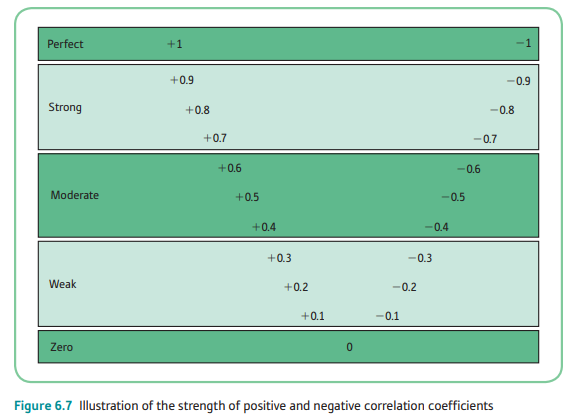
• A positive relationship simply means that high scores on x tend to go with high scores on y, and low scores on x tend to go with low scores on y, whereas a negative relationship means that high scores on x tend to go with low scores on y.

6.1.10 Variance Explanation of the Correlation Coefficient

Correlation Coefficient (r): a ratio between the covariance (variance shared by the 2 variables) and a measure of the separate variances

r = a measure of shared variance ÷ a measure of the separate variances

• A correlation coefficient is a good measure of effect size and can always be squared in order to see how much of the variation in scores on one variable can be explained by reference to the other variable.

6.1.11 Statistical Significance and Psychological Importance

• The correlation coefficient tells you how well the variables are related, and the probability value is the probability of that value occurring by sampling error.

• When you report your findings, report the correlation coefficient and think about whether r is meaningful in your particular study, as well as the probability value. Do not use the probability value on its own.

• REMEMBER: Statistical significance does not necessarily equal psychological significance.

6.1.12 Confidence Intervals around r

Rosnow and Rosenthal (1996) give the procedure for constructing 95% confidence limits (two-tailed p = 0.05) around r. The following is based on their text:

1. Consult a table to transform r to Fisher’s Zr.

2. Multiply 1/√(n - 3) by 1.96.

3. Find the lower limit of the confidence interval by subtracting the result in 2 above from the figure in 1.

4. Find the upper limit of the confidence interval by adding the result of 2 above to the figure in 1.

5. Consult a similar table to transform the lower and upper Zr values back to r values

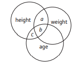
6.2 First- and Second-Order Correlations

Zero-Order Correlation: correlation between two variables without taking any other variables into account

Partial Correlation: can be explained by lookin at overlapping circles of variance; a correlation between two variables, with one partialled out

6.3 Patterns of Correlations

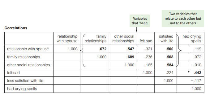
• If you look carefully, you can see that the variables that share most variance with each other have to do with quality of life – satisfaction with relationships and life. This is one pattern that you can see emerging from the data. These variables have correlated with each other; they form a natural ‘group’. The other two variables, ‘felt sad’ and ‘had crying spells’, also correlate with each other (0.442) – but not with the other variables – so this shows a second pattern. So, from these six variables, we can distinguish two distinct patterns. Obviously in this example, with so few variables, the patterns are relatively easy to distinguish.

• Psychologists who are designing or checking the properties of questionnaires make use of this ‘patterning’ to cluster variables together into groups. This is useful where a questionnaire has been designed to measure different aspects of, say, personality or quality of life.

• Using patterns of correlations to check that each set of questions ‘hangs together’ gives them confidence in their questionnaires.