Week 12 (Chapter 9)
Volatility and Volatility Models
Predicting the "volatility" of a financial variable is often of interest.
Conditional variance (or standard deviation) of a financial variable is commonly referred to as “volatility”.
AR(1) Model and Volatility
Conditional variance of a financial variable, commonly referred to ‘volatility’.
Recall a stationary AR(1) model: xt = ϕ0 + ϕ1x{t-1} + u_t.
Unconditional mean: E(xt) = \frac{ϕ0}{1 - ϕ_1}. (1)
The fraction arises from solving for long-run average of the series.
Conditional mean: E(xt|Ω{t-1}) = ϕ0 + ϕ1x_{t-1}. (2)
Unconditional variance: Var(xt) = \frac{σ^2}{1 - ϕ1^2}. (3)
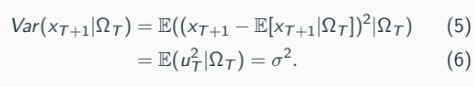
Conditional variance: Var(xt|Ω{t-1}) = σ^2, (4) where σ^2 = Var(ut|Ω{t-1}) = Var(u_t).
Unconditional variance is bigger in this model because it doesn't account for available information, unlike conditional variance (think of restricted and unrestricted model).
Forecasting with AR(1)
Forecast x{T+1} given ΩT
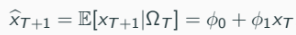
This is the conditional mean forecast.
ϕ0 and ϕ1 need to be estimated.
Conditional variance:
Assuming normality of ut:

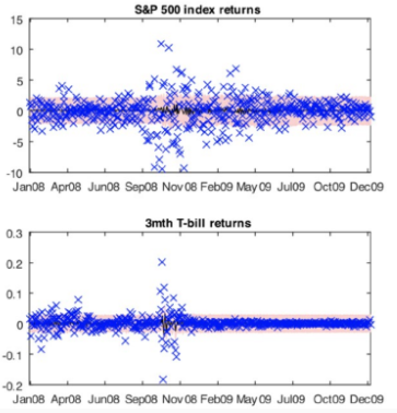
Forecasting example:
Blue: population observations
Black: conditional mean of the distribution
Pink: Forecast interval (95% CI)
Time series models are good at modeling time varying conditional mean, but if we are to assume TS4 for testing, then it contradicts to forecasting.
Conditional Distribution and Interval Forecasts
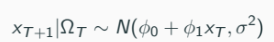
Conditional distribution of x{T+1} given ΩT depends on the distribution of u_t.
Assuming normality of ut: x{T+1}|ΩT \sim N(ϕ0 + ϕ1xT , σ^2). (7)
95% confidence intervals: ϕ0 + ϕ1x_T ± 2σ.
In practice, computed as: \hat{ϕ}0 + \hat{ϕ}1x_T ± 2\hat{σ}.
Issues with Constant Conditional Volatility
Constant conditional volatility assumption may not always hold.
In some periods, the assumption of conditional homoskedasticity performs poorly. For example, 20.8% of returns fall outside the 95% CI, while we'd expect only 5%.
Conditional homoskedasticity may not be a good assumption.
Time-Varying Conditional Mean vs. Variance
Time series models (e.g., AR(1)) are good at modeling time-varying conditional mean.
xt = ϕ1x{t-1} + ut
E[xt|Ω{t-1}] = ϕ1x{t-1} if E[ut|Ω{t-1}] = 0.
However, under conditional homoskedasticity, Var(ut|Ω{t-1}) = σ^2, which is constant over time, are not fit to explain variable of interest.
It is often necessary to allow “time-varying conditional variance” or “time-varying volatility”.
ARCH Models: Modeling Time-Varying Variance
Empirical evidence of time-varying conditional variance is seen in volatility clustering.
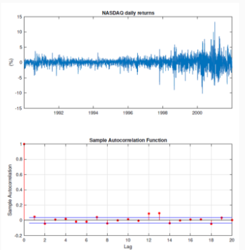
The time series is modeled as follow, xt = ϕ0 + ϕ1x{t-1} + u_t under conditional homoskedasticity.
Then estimate the model via OLS and obtain residuals \hat{u}t = xt − \hat{ϕ}0 − \hat{ϕ}1x_{t-1}.
Check if the conditional variance u_t is time-varying after obtain the time series residual.
Auto Regressive Conditional Heteroskedasticity (ARCH) Model
If the variance of ut doesn't look stable over time, the assumption Var(ut|Ω_{t-1}) = σ^2 is problematic.
ARCH(1) model:
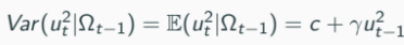
c represents a constant term, and γγ (gamma) represents the coefficient that measures the sensitivity of the conditional variance to the previous period's squared error term (ut−12)
This is an AR(1) framework for the time series of u_t^2.
Conditional variance is time-varying.
Conditional standard deviation is commonly referred to as “volatility”.
ARCH considers time-varying volatility of a financial variable (returns).
Details on ARCH Models
ARCH(1) model: E(ut^2 |Ω{t-1}) = c + γu_{t-1}^2 .
Volatility: \sqrt{c + γu_{t-1}^2}
The model is often written with a martingale difference sequence \etat w.r.t. Ωt.
\etat is a martingale difference sequence w.r.t. Ωt if E[\etat|Ω{t-1}] = 0.
ARCH(1): ut^2 = c + γu{t-1}^2 + η_t.
Generalizations:
ARCH(2): ut^2 = c + γ1u{t-1}^2 + γ2u{t-2}^2 + ηt
Value-at-risk
When portfolio returns are normally distributed, VaR tells us the investment loss at the first percentile of the return distribution (FINC2011).
Ignores the magnitudes of potential further losses.
In other words, 1% of the return portfolio may be viewed as worst-case scenario, so we test how much loss is from it.
VaR can be determined by mean and SD of the distribution:
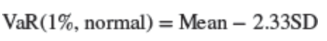
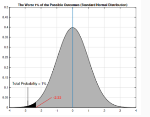
→ In conclusion: there is a 1% chance that portfolio value will fall by more than 2.33 (based on normal distribution).