Chapter 14-16

AGGREGATE DEMAND (Chapter 14):

AD = total spending on goods + services in a period of time at a given price level

on a graph = Price level v real GDP

• lower average price level = high average demand

Long Run Aggregate Demand (LRAD):

AD = C + I + G + (X - M)

• C -> consumption

  • durable vs non-durable goods

• I -> investments (producers)

  • replacement investment vs induced investment

• G -> government

• X -> exports

• M -> imports

Non-price determinants of Consumption: 

• Income taxes

  • higher income = higher consumption

  • higher income tax = lower consumption (less disposable income)

• Wealth

  • change in house prices / value of stocks and shares -> higher = higher consumption

• Interest Rates

  • higher interest rates = less borrowing -> lower consumption

  • lower interest rates = higher consumption (ceteris paribus)

• Consumer confidence / expectations of future

  • optimistic = higher consumption

  • consumer confidence index

  • higher future prices = higher consumption (vice versa)

• Debt

  • easy to borrow money + low interest = higher debt willingness + consumption 

  • hard to borrow money + high interest = lower debt willingness + consumption 

acronym: TWICED

Non-price determinants of Investments: 

• Interest rates

  • higher interest rate = lower investments

• Business confidence

  • optimistic about future = higher investments

• Technology

  • increase in tech = higher investments

• Business taxes

  • higher taxes = reduced post-tax profits = lower investments

• Corporate indebtedness

  • easy to borrow money + low interest = higher debt willingness + investment

  • hard to borrow money + high interest = lower debt willingness + investment

acronym: IB-TBC

Non-price determinants of Government Spending: 

• economic + political priorities

  • commitment to support industry = higher spending

  • correct market failure = higher spending

Non-price determinants of Net exports: 

• change in imports

  • higher domestic income = higher imports

  • higher exchange rate = higher imports

  • lower restrictions on trade = higher imports

  • lower inflation rates of foreign partners = higher imports

• change in exports

  • increased foreign incomes = higher exports

  • higher exchange rate of currency = lower exports

  • lower restrictions on trade = higher exports

  • higher inflation rate = lower exports

AGGREGATE SUPPLY (Chapter 15):

AS = total amount of goods + services produced by all industries at every given price level

Short Run Aggregate Supply (SRAS):

short run = period of time where FoP do not change

• wage / price of labour = fixed

• decrease in cost = higher supply

• positive relationship between price level and real GDP

Non-price determinants of SRAS:

1. Cost + availability of resources

   1. wage rates (increase in wages = increase in cost of FoP -> lower AS)

   2. cost of raw materials (higher costs = lower AS)

      1. dependent on how widely used the material is

   3. price of imports (increase in price = higher cost of production -> lower AS)

2. Government intervention

   1. subsidies (increased subsidies = higher AS)

   2. taxes (increased taxes = lower AS)

   3. regulations (more regulations = lower AS)

3. Supply shocks

   1. natural disasters

   2. wars / conflicts

Long Run Aggregate Supply (LRAS):

two schools of thought -> Keynesian vs neo-classical

Neo-classical:

• efficiency of market

• minimal gov intervention

• belief in invisible hand
  

• LRAS = perfectly inelastic

• full employment level

• independent of price level
  
  

Keynesian view:

1: AS is perfectly elastic

• spare capacity

• increase output without high costs

2: approaching potential output

• use up spare capacity

• FoP more scarce

• FoP cost more

• rising price levels

3: full capacity

• impossible to increase output

• AS perfectly inelastic

Non-price determinants: 

• Change in quantity or quantities of FoPs

• Technological improvements

• Increase in efficiency

• Changes in institutions

Factors influencing quality / quantity of FoPs:

MACROECONOMIC EQUILIBRIUM (Chapter 16):

Short run equilibrium

• when AD meets SRAS (AD = SRAS)

• no incentive for producers to increase output or prices

• no inflationary / deflationary pressure
  

Long run equilibrium

Neo-classical:

AD = LRAS

• economy always moves towards LRE without gov intervention

• changes to AD only on price level

Recessionary / Deflationary Gap

• equilibrium level of real output is less than potential output as result of decrease in AD (assumption = temporary)

Inflationary Gap

• equilibrium level of real output is more than potential output as result of increase in AD (assumption = temporary)

Growth / decrease of supply:

Long Run Equilibrium:

short run = inflationary and recessionary gaps exists

long run = equilibrium point must return to LRAS (full employment)

Keynesian:

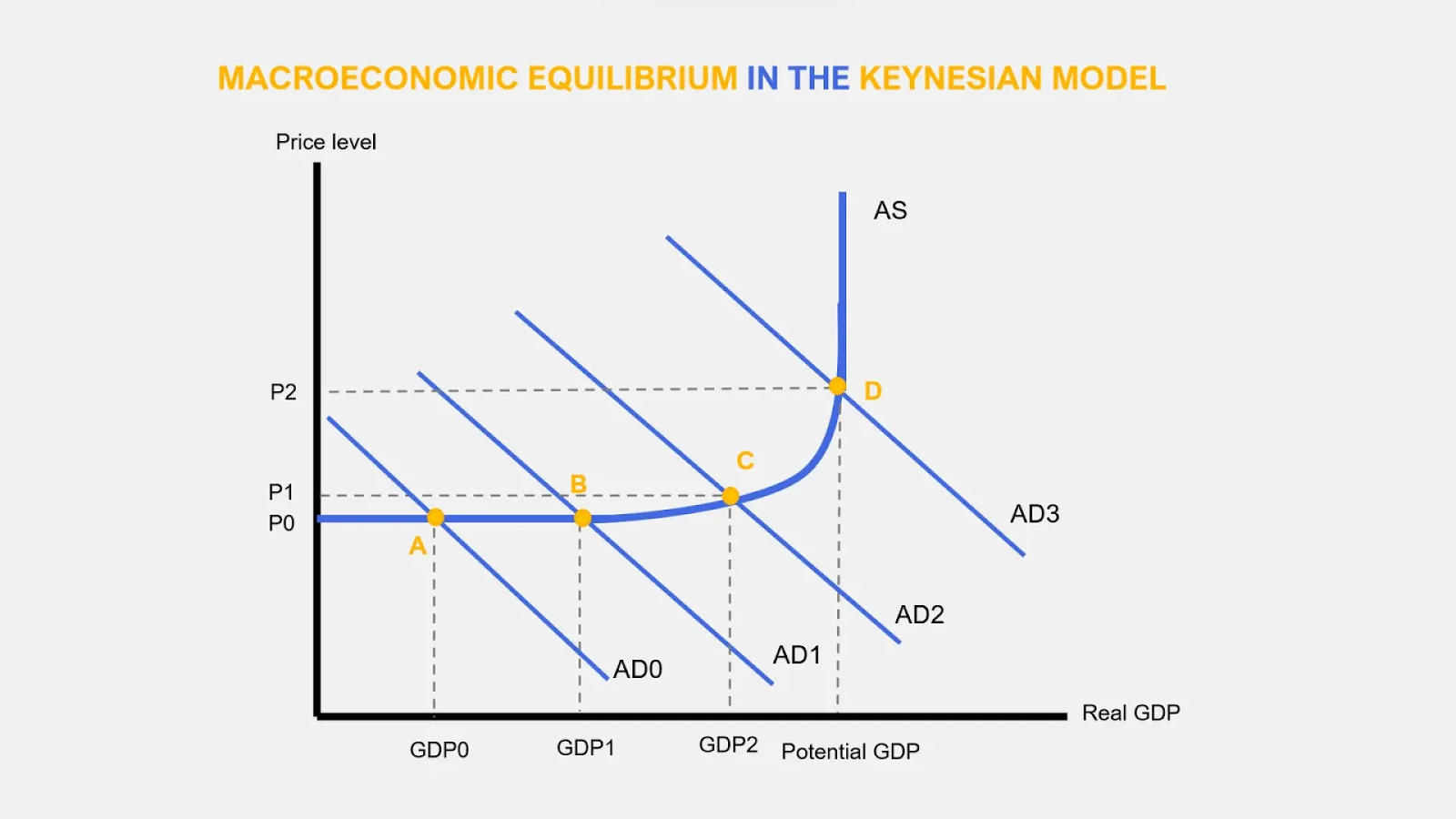
• economy may be in LRE at levels of output below full employment

• LRE depends on AD level

• AS = perfectly elastic -> spare capacity + unused FoP

• equilibrium below full employment level

first shift -> no change in price, only change in output

second shift -> slight inflationary pressure, increased price + output

third shift -> purely inflationary shift, only change in price, no change in output