AP Calculus BC: Unit 7 (ft. 6.13)

6.13 - Evaluating Improper Integrals

Infinite Intervals:

1. Limit

2. Replace inf with b (on top) or a (on bottom)

3. Find the antiderivative (u-sub, arctrig, etc.)

4. Subtract with bounds

5. If the answer is undefined (inf), DIVERGES

6. If the answer is a value, CONVERGES TO value

Infinite-Infinite Intervals:

1. Limit addition

   Integral (c/-inf) + integral (inf/c)

2. Replace -inf with a, inf with b

3. Antiderivative (u-sub, arctrig, etc.)

4. Subtract with bounds each of the two limits

5. If one diverges, it DIVERGES

6. If all answers are values, CONVERGES to the sum of values

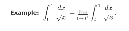
Infinite Discontinuities:

1. Identify the discontinuity (L or R)

2. Write the limit

3. Find the antiderivative

4. Subtract with bounds

5. Converges/Diverges

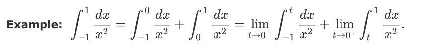
Infinite Discontinuities Internally

1. Identify the value that makes the integrand discontinuous

2. Limit to discontinuous value for both sides of c

3. Find antiderivative of each

4. If one diverges, it DIVERGES

5. If all answers are values, CONVERGES to the sum of values

7.1 - Modeling Situations with Differential Equations

Direct variation

Linear functions: y = kx

• y varies directly as x

• y is directly proportional to x

• y is “proportional” to x

Inverse variation

Function: y = k/x

• y varies inversely as x

• y is inversely proportional to x

Double check:

1. At a rate?

   dX/dt (assumed it’s over time)

2. K = constant of proportionality

3. Differences, sums, products, quotients

7.2 - Verifying Solutions for Differential Equations

Verifying solutions

1. Find the derivatives (1st, 2nd, 3rd…)

2. Plug in derivatives or y’s to differential equation

3. Check if it is a solution (= #) by setting them equal to each other

Double check:

1. When subtracting a group, multiply by negative 1 to each value

2. Solve for k

Differential equations

1. Write an equation of the tangent line to y = f(x)

   y - y₁ = m(x - x₁)

2. Use a tangent line to approximate a value of f(x)

   f(d) ≈ m(d - x₁) + y₁

3. Find d²y/dx²

   fig - fgi/g² (quotient rule)

   fig + fgi (product rule)

   Plug in for x and y terms

4. Find or check for critical values and relative extrema

   dy/dx = 0, derivative tests

Derivatives

1. Find out a squared value (always positive)

2. Find out how dy/dx can become negative (or positive)

3. State how dy/dx can be less (or greater) than 0

7.3 - Sketching Slope Fields

Sketching solution curves

1. Passing through a coordinate (x,y)

2. Stop at x-axis, BOTH sides

3. Range of solution curve y = f(x)

   [y₁, y₂], ex: [4,6] (in terms of y)

7.4 - Reasoning Using Slope Fields

Matching slope fields

• If slopes are the same vertically, only x

• If slopes are the same horizontally, only y

• If slopes have a combination, both x and y

Double check:

1. Plug in multiple coordinate points (x,y) to each equation

2. Process of elimination

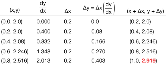
7.5 - Approximating Solutions Using Euler’s Method

Euler’s method

1. Separate variables (dy/dx)

2. Start at given point

   y(0) = 1

3. Plug in x and y into dy and multiply by dx (change in x, ∆x)

   dy = (x-y)dx = (0-1)(0.5) = -0.5

4. Add dy to original y for new y

   1 + (-0.5) = 0.5

5. Insert new y into new x (change in x, dx, ∆x)

   0 → 0.5 (∆x = 0.5), y = 0.5

6. y(1.5) ≈ 0.75; under approximation because d²y/dx² > 0 (plug in new y and new x)

   d²y/dx² = 1 - dy/dx = 1-(x-y) = 1-x+y = 1-1.5 + 0.75 > 0

Double check:

1. If f’’ > 0 → concave up, approxication is under (U)

2. If f’’ < 0 → concave down, approximation is over (n)

3. Approximation f(x) ≈

7.6 - Finding General Solutions Using Separation of Variables

Separating variables

1. Multiply dy/dx with dx

2. Divide y-variable

   y-values in left side, x-values in right side

3. Integrate (antiderivative)

4. Find y (square rooting, arctrig, e, etc.)

7.7 - Finding Particular Solutions Using Initial Conditions and Separation of Variables

Find particular solution

1. Multiply both sides of the equation by dx

2. Separate the variables (multiplying, dividing)

   y on left, x on right

3. Integrate both sides (u-sub, etc.)

4. Use initial condition to find C

   Plug in (x,y) to find C

5. Solve for y + C

6. Determine positive or negative when square rooting

   f(1) = -4

7.8 - Exponential Models with Differential Equations

Exponential Growth and Decay

y = Ce^kt

dy/dt = ky

• Growth: k > 0

• Decay: k < 0

• Half-lives of radioactive isotopes

  Ex: Carbon (¹⁴C) = 5730 years

Decay: Applications of half-life

Question: Suppose that 15 grams of caesium isotope Cs-137 that was released during the 1986 Chernobyl nuclear accident and absorbed into the groundwater. How long will it take for the 15 grams to decay to 1 gram and become safer to drink?

1. Plug in given (x,y)

   y = Ce^kt

   (0, 15) → 15 = Ce^k(0)

2. Find C

   15 = C

3. Plug in half-life (x,y)

   Caesium (¹³⁷Cs) = 30 years

   (30, 7.5) → 7.5 = 15e^k(30)

4. Find k (natural log)

   7.5 / 15 = 15e^k(30) /15

   ln(1/2) = ln(e^30k) → ln(1/2) /30 = 30k /30

   k = ln(1/2)/30

5. Plug in given to find t (log rules)

   y = 15e^ln(1/2)/30t → 1 = 15e^ln(1/2)*t/30

   1 /15 = 15(1/2)^t/30 /15

   ln(1/15) = ln(1/2)^t/30 → ln(1/15) /ln(1/2) = t/30*ln(1/2) /ln(1/2)

   ln(1/15)/ln(1/2) /30 = 30t /30

   t = 30*ln(1/15)/ln(1/2)* (don’t have to simplify if not given a calculator)

Growth: Application of population

Question: An absent-minded graduate student at a university is studying a population of fruit flies in a biology life. She works under the premise that this experimental population of fruit flies increases according to the law of exponential growth. She counts 100 flies after the second day of the experiment and 300 flies after the fourth day, however, she forgot to record the number of fruit-flies she initially had at the beginning of the experiment. Approximately how many flies were in the original population? Round to the nearest fly.

1. Plug in both given (x,y)

   y = Ce^kt

   100 = Ce^k(2) /e^2k, 300 = Ce^k(4) /e^4k

2. Find C by equalling both equations

   C = 100/e^2k, C = 300/e^4k

   100/e^2k = 300/e^4k → e^4k/e^2k = 300/100

   e^2k *ln = 3 *ln

3. Find k (natural log)

   ln(e^2k) = ln(3) → 2k /2 = ln(3) /2

4. Plug in found to find y (0,__)

   y = (100/e^2(ln(3)/2)e^ln(3)/2(0) → 100/3e⁰ → 100/3 flies ≈ 33 flies

Growth: More applications

Question: Fish are being introduced into a man-made lake. The rate of fish, F, with respect to time, t, is directly proportional to 900-F, where t is measured in years. When t=0, there are 400 fish in the lake and 3 years later, there are 600 fish in the lake.

1. Solving the differential equation, write the equation

   dF/dt *dt /900-F = k(900-F) *dt /900-F→ dF/900-F = kt

2. Integrate

   -ln|900-F| = kt +C, u=900-F du=-dF

3. Solve for C by plugging in a point (x,y)

   (0,400) → -ln|900-400| = k(0) +C → -ln|500| = C

4. Solve for k by plugging in C and plugging in another point (x,y)

   (3, 600) → -ln|900-600| +ln|500| = k(3) - ln|500| +ln|500|

   ln|500/300| /3 = k(3) /3 → ln|5/3|/3 = k

5. Isolate F by plugging in known values

   -ln|900-F| *-1 *e = 1/3ln(5/3)t - ln|500| *-1 *e

   F = 900-e^{-1/3ln(5/3)t + ln(500)}* (do not have to simplify)

6. Find the fish population in another 3 years

   t = 6, F(6) = 900-500(3/5)^6/3 = 720 fish

7. Find lim (t→inf)F(t) and explain what the answer means

   lim(t→inf) (900-500(3/5)^t/3) = 900-0=900

   The maximum number of fish that could inhabit the lake would be 900 fish.

7.9 - Logistic Models with Differential Equations

Logistic differential equation form

dy/dt = ky(1-y/L)

Logistic growth equation form

y = L/1+be^-kt

Double Check:

• L = carrying capacity

• k = growth constant

• k is negative in growth form