Week 3 Project Analysis

Page 3: Capital Investments

Items for consideration

Establish capital budgeting processes for orderly investment decisions.

1. Preparation of Capital Budget

   • List investment projects aligned with strategic plans.

   • Consistent project development is crucial.

2. Submission of Appropriation Request

   • Include forecasts, discounted-cash-flow analysis, and supporting information.

3. Potential Biases

   • Be wary of sponsors overstating cash flows and understating risks led to bias forecast.

   • Avoid offsetting optimistic forecasts with "fudge factors".

4. Post Audits

   • Review project outcomes against forecasts, how close they are and if expectations are met.

   • Identify issues and learn from mistakes.

Page 4: Handling Uncertainty

Good Capital Budgeting Practices is to be able to identify major uncertainties in projects. Since cash flow estimates for projects are uncertain; methods below provide ways to handle such uncertainty.

Methods for Handling Uncertainty

• Sensitivity Analysis

  • Analyze how NPV is affected by variable changes (only one variable at a time, e.g. sales, costs, etc.).

• Scenario Analysis

  • Evaluate specific combinations of variable changes.

• Simulation Analysis

  • Estimate probabilities of different outcomes and generate a probability distribution for NPV.

• Break-Even Analysis

  • Determine the level of sales where a company breaks even.

Page 5: Sensitivity Analysis

Overview

• Examines the impact of variable changes on project NPV (only one variable is changed at a time).

Benefits

• Easy to carry out on a spreadsheet program.

• Expresses cash flows in relation to key variables and help calculating the consequences of misestimating the variables.

• Helps managers identify key variables needing further information, identify the most useful and help expose inappropriate forecast.

• Can recompute NPV using expected, pessimistic, and optimistic estimates of variables.

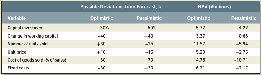
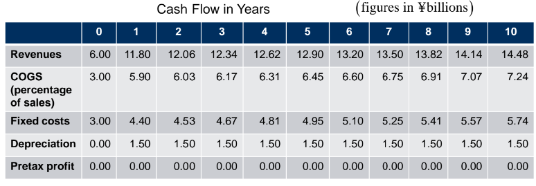
Page 6: Otobai Sensitivity Analysis Example

Project Overview

• Product: High-performance electric scooter.

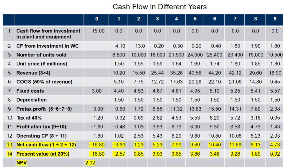
• Initial Findings: NPV of ¥2.02 billion at a 20% opportunity cost of capital.

  • Increasing investments in net working capital as sales build.

  • COGS set at 50% of sales, alongside fixed costs.

  • Tax at 40%, post-depreciation.

• After year 6: sales to tail off as more competitions enter the market, price of scooter might be reduced.

Objectives

• Analyze cash flow forecasts and identify key value drivers for project success or failure.

Strategy

• Analyze investment in plant and working capital and forecast sales volume, price and costs of the projects.

• Engage marketing and production staff to generate optimistic and pessimistic estimates for each of the underlying variables.

• Recalculate NPV using varying estimates for key variables.

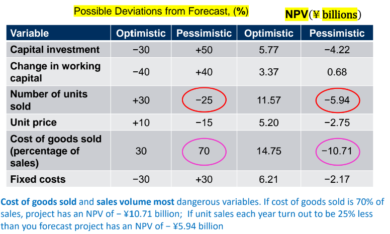
Key Findings

• Most sensitive variables: COGS and sales volume.

• Significant downside potential with higher COGS or lower sales.

Visualization Tool

• A tornado diagram illustrates the impact of variable uncertainty on NPV.

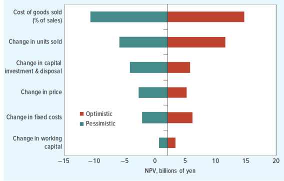
Insights

• Cost of goods sold, and sales volume show the greatest variability, as the range of NPV outcomes varies, as shown at the summit of the tornado.

• Fixed costs and working capital have a more modest effect on NPV.

Page 12: Limitations of Sensitivity Analysis

Key Challenges

• Ambiguity in defining optimistic and pessimistic scenarios.

• Requires subjective probability distributions, hard to derive.

• Underlying variables may be interrelated (e.g. inflation affects costs).

• Sensitivity analysis does not give NPV for the likely bad or good overall outcomes.

Suggested Solution

• We can get around this problem by defining underlying variables that are roughly independent. However, we can’t push one-at-a-time sensitivity analysis too far.

• Scenario Analysis is recommended for consistent variable interactions.

Page 13: Scenario Analysis

Overview

• Develops plausible future scenarios that have uncertain developments that may impact major investment projects.

• Encourages companies to rely on comprehensive examination of potential environmental changes in the future.

Comparison to Sensitivity Analysis

• Involves multiple variable interactions rather than single-variable changes.

• Focuses on major, mutually consistent changes rather than best/worst outcomes.

Page 14: Break-Even Analysis

Objective

• Assess the extent of adverse developments needed to drive NPV to zero, if the future turns out worse than forecast, the company would love to save those loss.

• Identify thresholds for different variables using break-even points.

Page 15: Break-Even Point Analysis

Look where NPV turns negative, defines break-even point at which NPV is 0.

Excel method for break-even point analysis (What If Analysis):

Data → Goal Seek → Set Cell [] → To value [0] → By changing cell []

A project’s accounting break-even point is the minimum level of sales required to avoid an accounting loss.

Page 17: Operating Leverage

Definition

• The extent to which fixed costs influence profit changes due to sales fluctuations.

Measurement

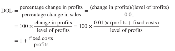
• Degree of Operating Leverage (DOL): Reflects the percentage profit change for a 1% sales change.

  

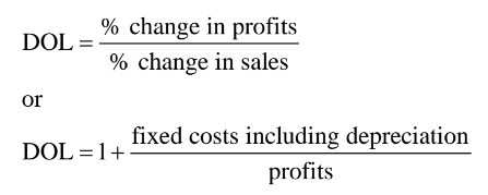
Understanding DOL Calculation

• If sales rise by 1%, then variable costs will also increase by 1%, profit will increase by 0.01 x (sales - variable costs) = 0.01 x (pretax profits + fixed costs).

  

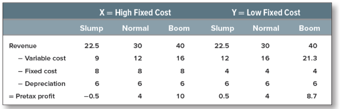
• In normal times, both companies (X and Y) earn the same profit, however, higher fixed costs suffer sale volume in slump and gain more in a boom. DOL for Y is 3.5. Dol for X is 4.5.

Page 21: Monte Carlo Simulation

Overview

• Extends sensitivity analysis by exploring all variable combinations.

• Useful when a limited number of scenarios and combinations of variables are considered.

• Provides a comprehensive output distribution for the project outcomes.

Steps in the Monte Carlo Modeling Process

1. Build a detailed financial model for cash flows, involving a set of equations for each variable that determines cash flow.

2. Specify probability distributions (frequency) for variables by specifying probabilities for errors in forecasts.

3. Simulate cash flows based on forecast error distributions in order to calculate cash flows for each period.

4. Calculate NPV from simulated cash flows.

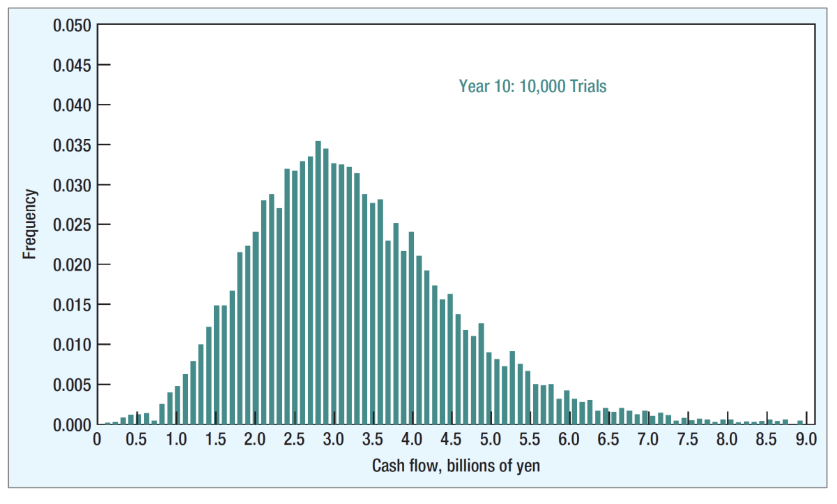
→ The likely outcomes is 3.4 billions yen.

→ Each uncertain variables here has a unique frequency/distribution.

→ Run simulation on thousands of trials.

1. Identify the Best NPV:

   • Look for the NPV values that are most frequent in the distribution and those that provide a favorable range for decision-making. The best NPV is generally considered to be:

     • The highest value of NPV, indicating the most profitable investment.

     • Analyze the probability of achieving this NPV, which can be expressed in terms of percentiles (e.g., the 50th percentile represents the median NPV).

2. Consider Risk: Assess the spread of the NPV outcomes. A high standard deviation may indicate higher risk, even if the average NPV is attractive.

3. Explanation Strategy:

   • When explaining your findings, discuss the significance of NPV as a financial metric, describe how you ran the Monte Carlo simulation, summarize the outcomes, highlight the most favorable NPVs, and address the associated risks based on the distribution of results. Use visual aids like graphs to effectively convey the information and support your conclusions.

Page 24: Flexibility & Real Options

Real Options Overview

• DCF analysis assumes passive asset management, which is not realistic. Since manager will not be passive after investing in a new project.

  • Project maybe expanded, cut back or abandoned altogether.

• Real options offer adaptability in project management based on unfolding circumstances.

• Options to modify projects, flexibility in a project, are known as real options.

Value of Flexibility

Flexibility enhances a project’s value, particularly in uncertain scenarios.

Real options derive their value from managerial flexibility in the size, timing and nature of the investment in an uncertain world.

→More uncertainty means more flexibility in the project’s plan means more valuable the project is.

Page 25: Types of Real Options

1. Option to Expand: Future possibilities for expansion.

2. Option to Abandon: Cease or sell unprofitable projects.

3. Production Options: Flexibility to adjust production inputs/outputs adapt to demand.

4. Timing Options: Adjust investment timing to market conditions, able to postpone or bring forward.

Page 26: Option to Expand

Strategic Flexibility

• Open pathways for future growth based on evolving market conditions.

Examples

• Investing in smaller-scale projects with potential for expansion.

Page 27: Option to Abandon

Exit Strategies

• Cease operations on unprofitable projects to minimize losses.

• cut losses, reallocate resources to a better opportunity, exit a project under adverse condition.

• Tangible assets are usually easier to sell than intangible ones.

Examples

• Shutting down a failing product line.

Page 28: Production Real Options

Input/Output Variability

• Adjust production based on market demand and costs.

• Allow firms to manage uncertainty, optimize resource allocation, and respond strategically to changing market and economic condition.

Examples

• Flexible manufacturing systems allowing for swift product changes.

Page 29: Timing Real Options

Investment Timing Flexibility

• Options to optimize project timing based on market factors.

• Initiate, defer, accelerate, or abandon projects based on evolving market conditions, technological advancements, or else.

Examples

• Delaying product launches or scaling operations as needed.

Page 30: Decision Trees

Overview

• Sequential decision-making diagrams to visualize project choices.

Value of Decision Trees

• Helps assess real options and potential project outcomes.

Page 32: Pharmaceutical R&D Decision Tree Example

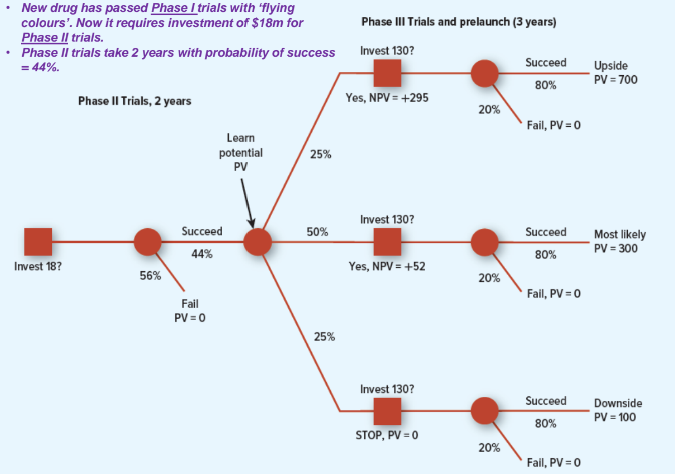
NPV Calculations

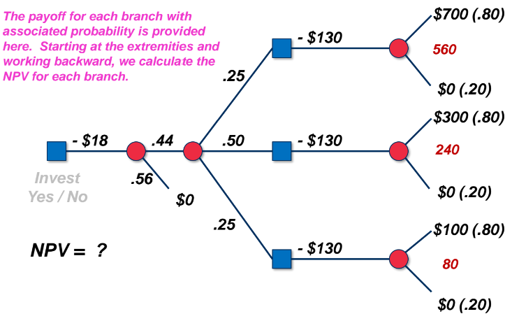
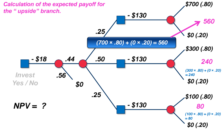
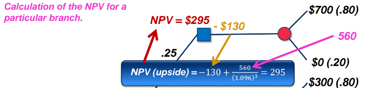
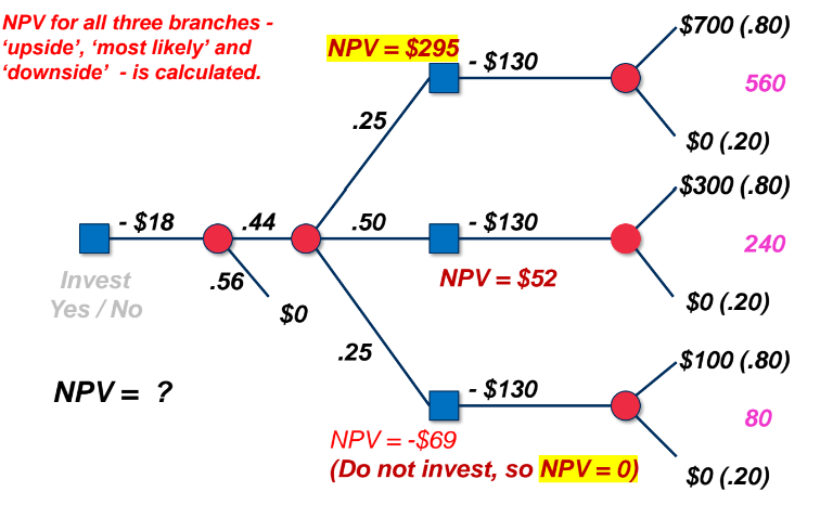
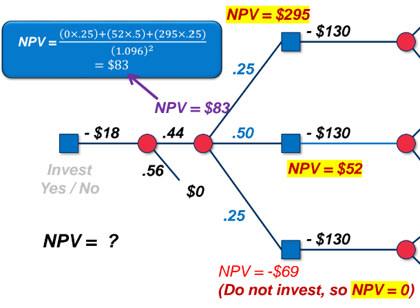
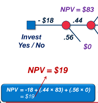
→ Since NPV is positive, we should invest in this project.