Ch3 Decision Analysis

Chapter Outline:

3.1 The Six Steps in Decision Making

3.2 Types of Decision-Making Environments

3.3 Decision Making Under Uncertainty

3.4 Decision Making Under Risk

3.5 Using Software for Payoff Table Problems

3.6 Decision Trees

3.7 How Probability Values Are Estimated by Bayesian Analysis

3.8 Utility Theory

Introduction

• Definition of Good Decision-Making:

  • Involves logic and rationality.

  • Considers available data and alternatives.

  • Applies quantitative approaches to analysis.

The Six Steps in Decision-Making

1. Define the problem: Clearly articulate the issue being faced.

2. List possible alternatives: Identify options available to solve the problem.

3. Identify possible outcomes: Recognize potential states of nature resulting from each alternative.

4. List payoffs: Determine the profit (or other measures) associated with each alternative-outcome combination.

5. Select a decision model: Choose an appropriate mathematical model for analysis.

6. Apply the model: Implement the chosen model and make a final decision.

Case Study: Thompson Lumber Company

Problem Definition

• Objective: Expansion by developing backyard storage sheds.

Step-by-Step Decision Making

• Alternatives:

  • Construct a large plant.

  • Construct a small plant.

  • Do not develop the new product line.

• Possible Outcomes:

  • Market condition could be favorable or unfavorable.

Payoff Values and Decision Models

Payoff Table for Thompson Lumber

• Note: Include all alternatives, even "do nothing."

Types of Decision-Making Environments

1. Decision Making Under Certainty:

   • Outcomes and consequences are known.

   • The decision maker knows with certainty the
     consequences of every alternative or decision choice

2. Decision Making Under Uncertainty:

   • Probabilities of outcomes are unknown.

   • The decision maker does not know the probabilities of the various outcomes

3. Decision Making Under Risk:

   • Probabilities of outcomes are known.

   • The decision maker knows the probabilities of the various outcomes

Decision Making Under Uncertainty

Decision Criteria

1. Maximax: Optimistic choice maximizing maximum payoffs.

2. Maximin: Pessimistic choice maximizing minimum payoffs.

3. Criterion of Realism (Hurwicz):

   • Weighted average between optimistic and pessimistic.

   • Often called weighted average
     –Compromise between optimism and pessimism
     –Select a coefficient of realism α, with 0 ≤ α ≤ 1
     α = 1 is perfectly optimistic
     α = 0 is perfectly pessimistic
     –Compute the weighted averages for each alternative
     –Select the alternative with the highest value
     Weighted average = α(best in row)
     + (1−α)(worst in row)

4. Equally Likely (Laplace):

   • Treat all outcomes equally likely and select based on average payoffs.

   • Considers all the payoffs for each alternative
     –Find the average payoff for each alternative
     –Select the alternative with the highest average

5. Minimax Regret:

   • Minimize potential regret from not choosing the best alternative.

   • Based on opportunity loss or regret
     –The difference between the optimal profit and
     actual payoff for a decision
     1. Create an opportunity loss table by
     determining the opportunity loss from not
     choosing the best alternative
     2. Calculate opportunity loss by subtracting each
     payoff in the column from the best payoff in
     the column
     3. Find the maximum (best) opportunity loss for
     each alternative and pick the alternative with
     the minimum (worst) number

Maximax Criterion Example (Thompson)

Maximin Criterion Example (Thompson)

Criterion of Realism Example (Thompson)

• Weighting Factor (α): 0.8

Calculations

• For Large Plant:

  Weighted Average = (0.8)(200,000) + (0.2)(-180,000) = 124,000

• For Small Plant:

  Weighted Average = (0.8)(100,000) + (0.2)(-20,000) = 76,000

Equally Likely Criterion Example (Thompson)

Average Payoffs

Example - Kenneth Brown (1/2)

• Analysis of Equipment Purchases:

  • Alternatives: Sub 100, Oiler J, Texan.

  • Market Conditions: Favorable vs. Unfavorable.

Minimax Regret Analysis

1. Construct Opportunity Loss Table.

2. Select Minimum Regret Alternatives:

Example Payoffs and Losses

Decision Making Under Risk

• Objective: Maximize Expected Monetary Value (EMV).

• When there are several possible states of nature and the
  probabilities associated with each possible state are
  known
  –Most popular method – choose the alternative with the
  highest expected monetary value (EMV)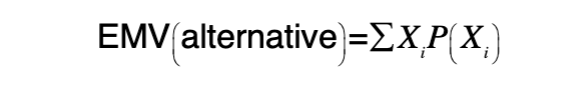

  

  where
  Xi = payoff for the alternative in state of nature i
  P(Xi) = probability of achieving payoff Xi (i.e., probability of
  state of nature i)
  ∑ = summation symbol i=1 to n (Xi * P(Xi)) where n is the total number of possible states of nature.

• Expanded Form of Expected Monetary Value
  EMV (alternative i) = (payoff of first state of nature)
  ×(probability of first state of nature)
  + (payoff of second state of nature)
  ×(probability of second state of nature)
  + ... + (payoff of last state of nature)
  ×(probability of last state of nature)

EMV Calculation

EMV = Σ(P(Xi) * Payoff) where P(Xi) = probability of state of nature i.

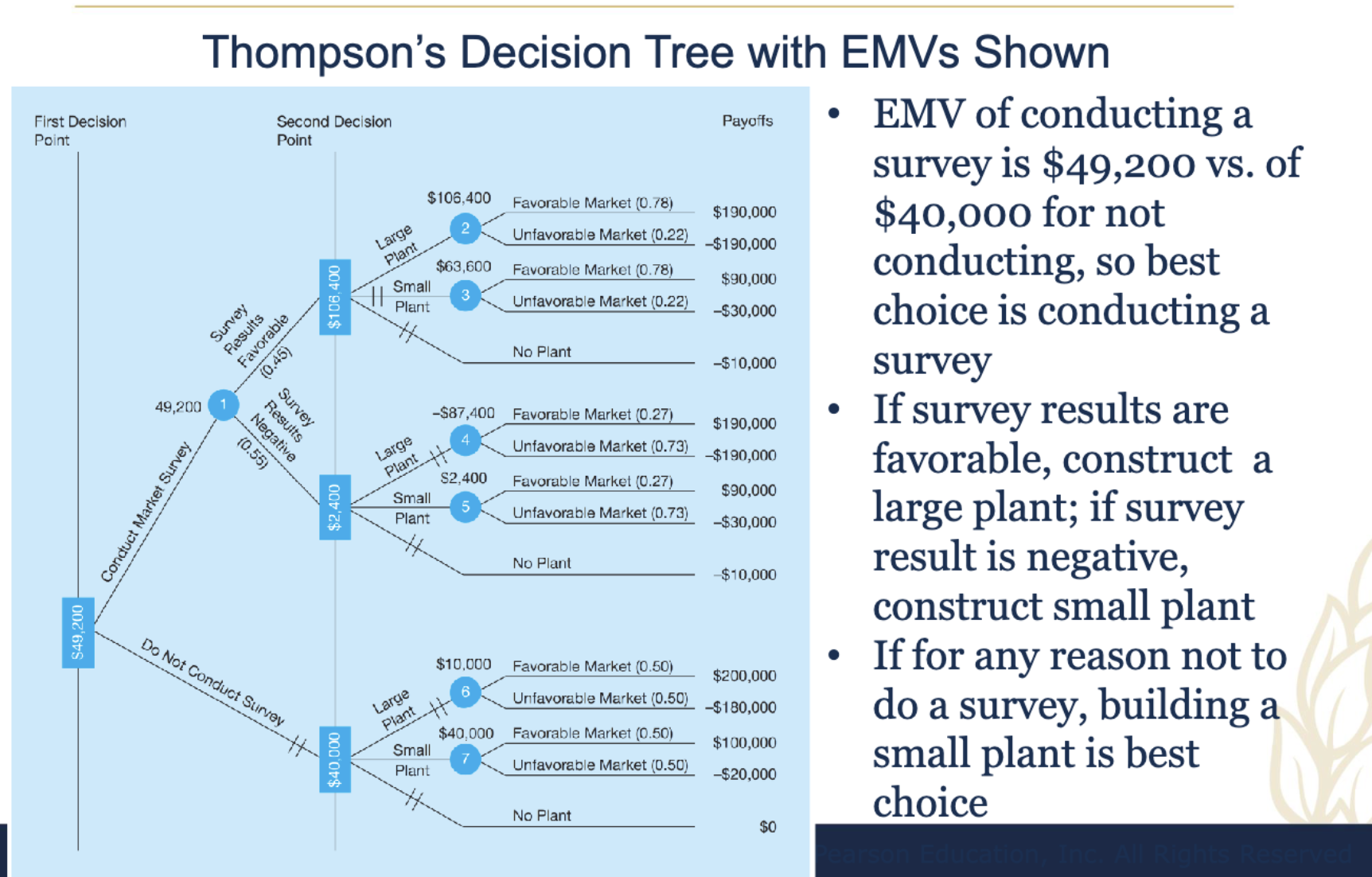
Critical Example - Thompson Lumber EMV

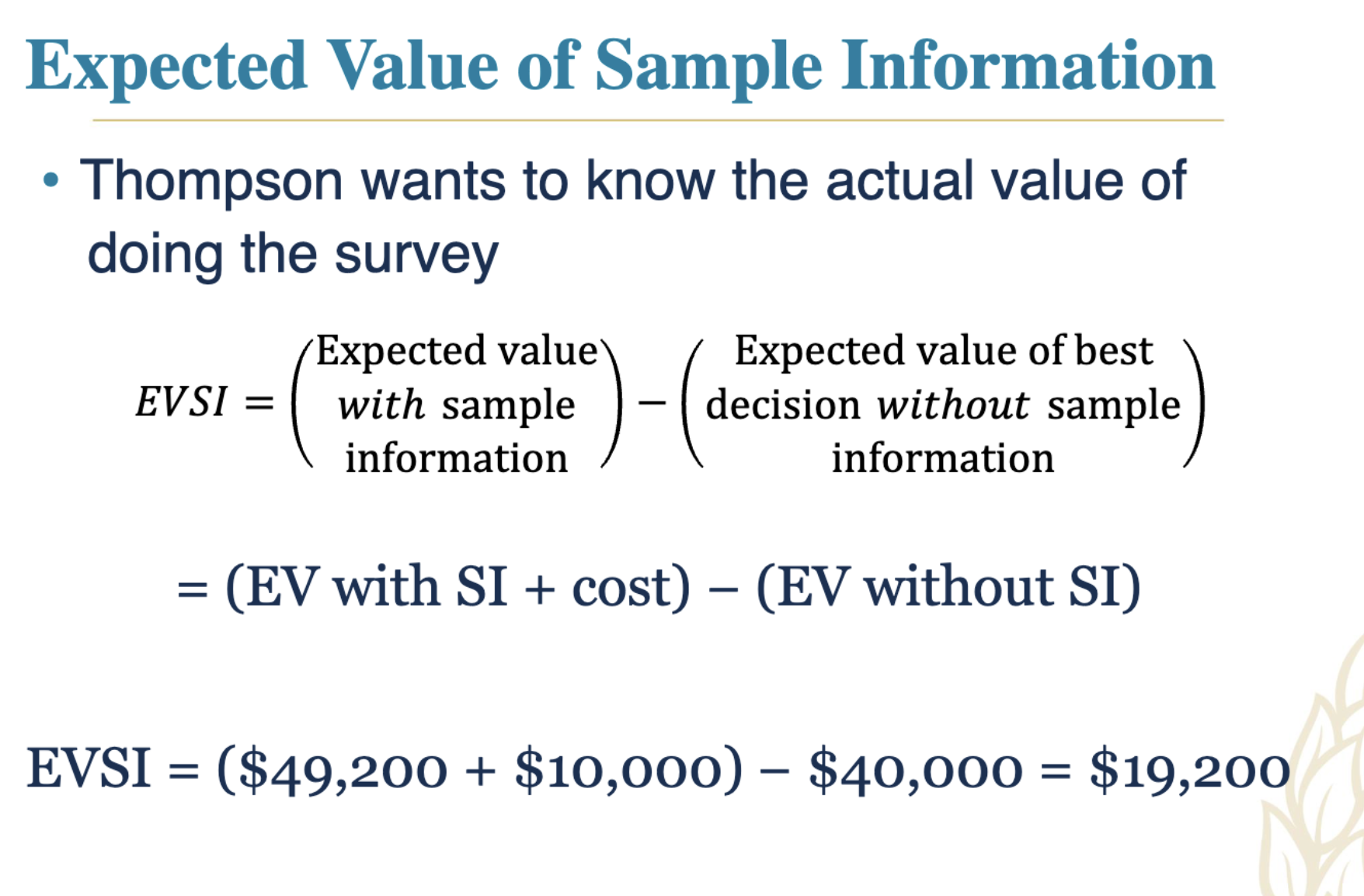
Expected Value with Perfect Information (EVwPI)

EVwPI = Σ(best payoff in state i) * P(state i)

Expected Value of Perfect Information (EVPI)

EVPI = EVwPI - Best EMV

• Example Application with Cost Analysis.

Expected Opportunity Loss (EOL)

EOL Calculation Method

EOL = Σ(Opportunity Loss * P)

3:6 Decision Tree

Any problem that can be presented in a decision table can
be graphically represented in a decision tree
–Most beneficial when a sequence of decisions must be
made
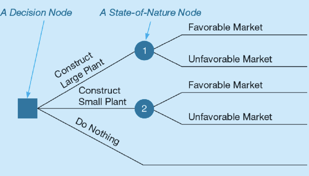
–All decision trees contain decision points/nodes
and state-of-nature points/nodes
–At decision nodes, one of several alternatives may be
chosen
–At state-of-nature nodes, one state of nature will occur

Steps of Decision Tree

1. Define the problem
2. Structure or draw the decision tree
3. Assign probabilities to the states of nature
4. Estimate payoffs for each possible combination
of alternatives and states of nature
5. Solve the problem by computing expected
monetary values (EMVs) for each state of
nature node

Structure of Decision Tree

• Trees start from left to right
• Trees represent decisions and outcomes in sequential
order
• Squares represent decision nodes
• Circles represent states of nature nodes
• Lines or branches connect the decision nodes and the
states of nature

Utility Theory Overview

• Utility reflects the overall value of decision outcomes beyond monetary value.

Decisions aim to maximize utility, characterized by risk preferences.

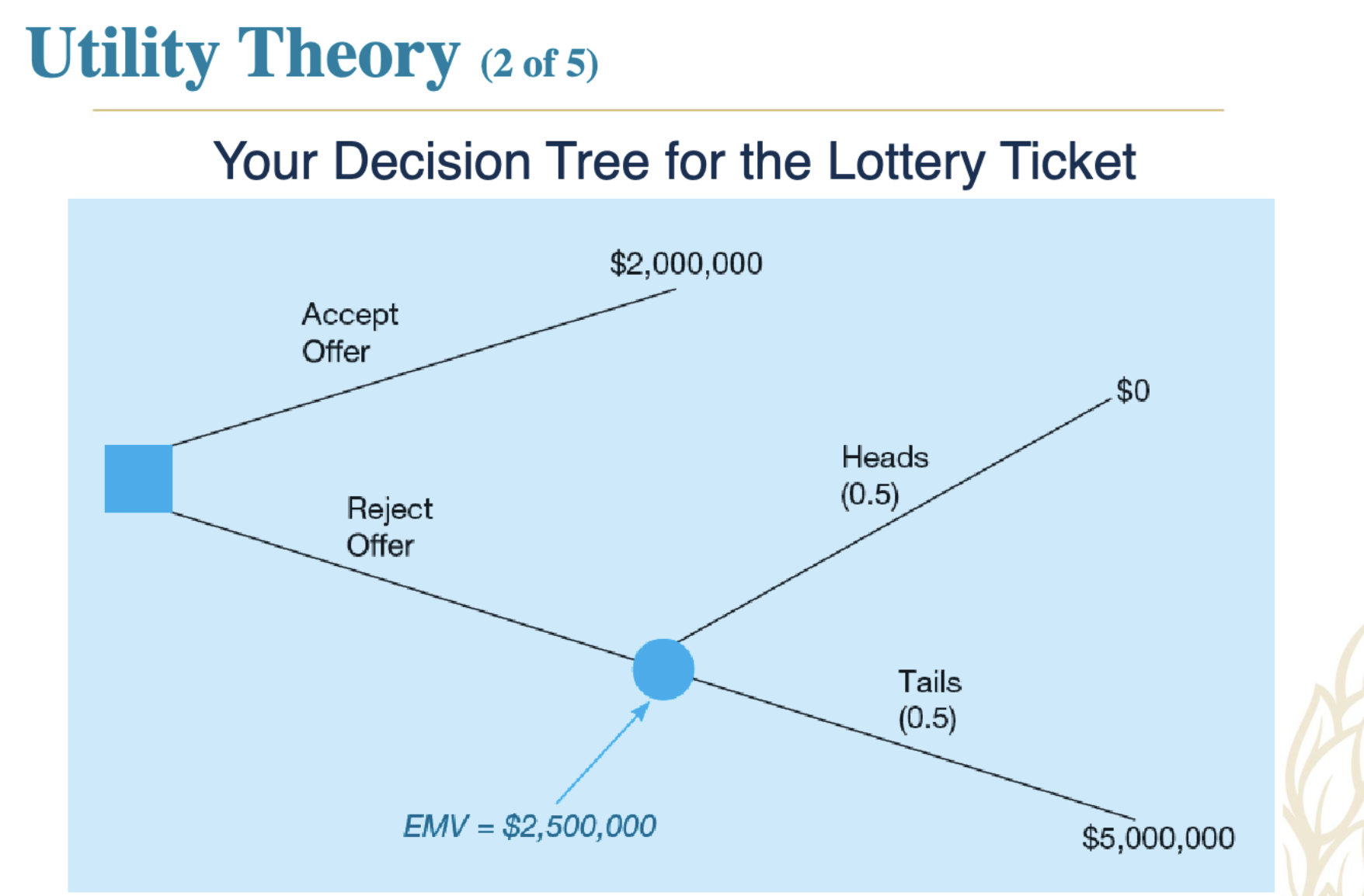
Utility assessment assigns the worst outcome a
utility of 0 and the best outcome a utility of 1
• A standard gamble is used to determine utility
values
• When you are indifferent, your utility values are
equal

Expected utility of alternative 2
= Expected utility of alternative 1
Utility of other outcome
= (p)(utility of best outcome, which is 1)
+ (1−p)(utility of the worst outcome, which is 0)
Utility of other outcome
= (p)(1) + (1−p)(0) = p

Key Takeaways

• Decision-making incorporates a range of strategies depending on certainty and available information.

• The choice of model affects outcomes significantly, emphasizing a need for careful analysis.