Theme 1

Rigid-Body Kinematics

Rigid-body kinematics: studies the relationships between linear and angular motions of bodies, disregarding forces and moments. It is crucial in designing gears, cams, connecting links, and other moving machine parts.

Rigid-Body Assumption

A rigid body is defined as a system of particles where distances between particles remain constant.

• In reality, all solid materials deform under force.

• The rigid-body assumption is valid when deformations are small compared to the overall body movement.

  • Example: Aircraft wing flutter doesn't affect the overall flight path.

• The assumption is invalid if deformations are significant and under study.

  • Example: Analyzing internal wing stress due to flutter requires considering relative motions within the wing.

Plane Motion

Plane motion occurs when all parts of a rigid body move in parallel planes. Typically, the plane of motion contains the mass center, treating the body as a thin slab.

Types of Plane Motion (Fig. 5/1)

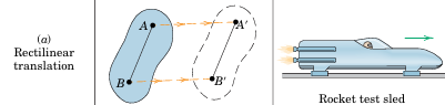
1. Translation: Every line in the body remains parallel to its original position; no rotation occurs.

   • Rectilinear Translation (a): All points move in parallel straight lines.

     • Example: Rocket test sled.

   

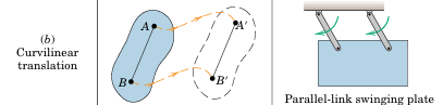
   • Curvilinear Translation (b): All points move on congruent curves (All points on the rigid body move along curves that are identical in shape and size. Essentially, if you were to trace the paths of different points on the body, each path would be the same curve, just shifted in position.).

     • Example: Parallel-link swinging plate.

   

   • Translation is fully defined by the motion of any single point in the body as all points share the same motion.

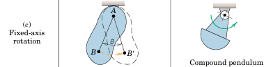
2. Rotation about a Fixed Axis (c): Angular motion around the axis. All particles move in circular paths, and lines perpendicular to the axis rotate through the same angle in the same time.

   • Example: Compound pendulum.

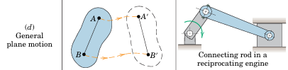
3. General Plane Motion (d): A combination of translation and rotation. Relative motion principles (Art. 2/8) are used to describe it.

• Example: Connecting rod in a reciprocating engine.

Analysis Methods

Plane motion analysis can be performed by:

1. Directly calculating absolute displacements and their time derivatives from geometry.

2. Utilizing principles of relative motion.

Rotation

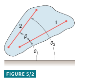
Rotation is described by angular motion. In Fig. 5/2, lines 1 and 2 on a rotating body have angular positions 𝜃_1 and 𝜃_2 from a fixed reference. The angle 𝛽 between the lines is constant.

• Relationship: 𝜃_2=𝜃_1+𝛽

• Differentiation yields: \dot{\theta_2} = \dot{\theta_1} and \ddot{\theta_2} = \ddot{\theta_1} or during a finite interval, \Delta\theta_2=\Delta\theta_1.

• All lines on a rigid body in plane motion share the same angular displacement, angular velocity, and angular acceleration. Angular motion depends on angular position relative to a fixed reference and its time derivatives. It does not require a fixed axis.

Angular-Motion Relations

Angular velocity \omega and angular acceleration \alpha are the first and second time derivatives of angular position \theta:

• \omega = \frac{d\theta}{dt} = \dot{\theta}

• \alpha = \frac{d\omega}{dt} = \dot{\omega} or \alpha = \frac{d^{2}\theta}{dt^{2}} = \ddot{\theta}

• \omega d\omega = \alpha d\theta or \dot{\theta} d\dot{\theta} = \ddot{\theta} d\theta

These equations are analogous to rectilinear motion equations (Eqs. 2/1, 2/2, and 2/3).

Constant Angular Acceleration

Integrating the above equations with constant angular acceleration gives:

• \omega = \omega_{0} + \alpha t

• \omega^{2} = {\omega_0}^{2} + 2\alpha (\theta - \theta_0)

• \theta = \theta_0 + \omega_0t + \frac{1}{2} \alpha t^{2}

Where:

• \theta_0 and \omega_0 are initial angular position and velocity at t = 0.

• t is the duration of motion.

Graphical relationships for s, v, a, and t (Figs. 2/3 and 2/4) can be applied to \theta, \omega, and \alpha by substitution.

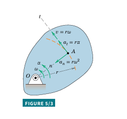
Rotation about a Fixed Axis

Points on a rigid body rotating about a fixed axis (Fig. 5/3) move in concentric circles (share the same centre). The relationships between linear motion of a point and angular motion of the body are:

• v = r\omega

• a_{n} = r\omega^{2} = \frac{v^{2}}{r} = v\omega

• a_{t} = r\alpha

Where:

• v is the tangential velocity.

• a_{n} is the normal acceleration.

• a_{t} is the tangential acceleration.

• r is the radius of the circular path.

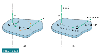
Vector Formulation

Using the right-hand rule (Fig. 5/4a), the angular velocity vector \overline{\omega} is normal to the plane of rotation. The linear velocity \overline{v} is obtained by:

• \overline{v}=\dot{\overline{r}}=\overline{\omega}\times\overline{r}

The vector equivalents to the scalar equations are:

• \overline{v}=\overline{\omega}\times\overline{r}

• \overline{a}_{n}=\overline{\omega}\times(\overline{\omega}\times\overline{r})=\overline{\omega}\times\overline{v}

• \overline{a}_{t}=\overline{\alpha}\times\overline{r}

Where \overline{\alpha}=\dot{\overline{\omega}} is the angular acceleration vector. However, for three-dimensional motion, \omega may change in direction, and \alpha will not necessarily be in the same direction as \omega.

The acceleration of point A is obtained by differentiating the cross-product expression for v:

• \overline{a}=\dot{\overline{v}}=\overline{\omega}\times\dot{\overline{r}}+\dot{\overline{\omega}}\times\overline{r}=\overline{\omega}\times(\overline{\omega}\times\overline{r})+\dot{\overline{\omega}}\times\overline{r}=\overline{\omega}\times\overline{v}+\overline{\alpha}\times\overline{r}

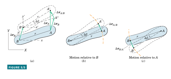
Relative Velocity Due to Rotation

For two points on the same rigid body, the motion of one point observed from the other is circular because the distance between them is constant. Figure 5/5a illustrates a rigid body moving from AB to A'B' in time \Delta t. This can be visualized in two steps:

1. Translation to A''B' with displacement \Delta r_{B}.

2. Rotation about B' through angle \Delta \theta, resulting in displacement \Delta r_{A/B}.

An observer at B' sees A undergoing fixed-axis rotation about B (Fig. 5/5b). The relationships for circular motion (Arts. 2/5 and 5/2) describe the relative motion of point A.

The total displacement of A is:

\Delta r{_{A}}=\Delta r_{B}+\Delta r_{A/B}

Dividing by \Delta t and taking the limit as \Delta t approaches zero gives the relative-velocity equation:

v_{A}{}=v_{B}+v_{A/B}

With the magnitude of the relative velocity being:

v_{A/B} = r\omega

In vector form:

\overline{v}_{A/B}=\overline{\omega}\times\overline{r}

Where \omega is the angular-velocity vector normal to the plane of motion. The relative linear velocity is always perpendicular to the line joining the two points.

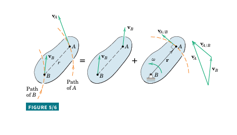
Interpretation of the Relative-Velocity Equation

Figure 5/6 emphasizes the translation and rotation components of the equation. The velocity of A is the vector sum of the translation portion \overline{v}_{B} plus the rotational portion \overline{v}\overline{}_{A/B}=\overline{\omega}\times\overline{r} .     The relative linear velocity is perpendicular to the line joining the points.

Solution of the Relative-Velocity Equation

Solved via scalar or vector algebra, or graphically. A vector polygon helps visualize physical relationships.

• Scalar components are obtained by projecting vectors. Simultaneous equations can be avoided with careful selection of projections.

• Alternatively, i- and j- components can be used, resulting in two scalar equations.

• Graphical solutions are useful for awkward geometries.

Relative Acceleration

Differentiating the relative-velocity equation with respect to time gives the relative-acceleration equation:

\overline{a}_{A}=\overline{a}_{B}+\overline{a}_{A/B}

Where a_{A/B} is the acceleration of A relative to B as seen by a nonrotating observer moving with B.

Relative Acceleration Due to Rotation

If A and B are on the same rigid body, A has circular motion about B, so a_{A/B} has normal and tangential components:

\overline{a}_{A}=\overline{a}_{B}+(\overline{a}_{A/B})_{n}+(\overline{a}_{A/B})_{t}

Where:

• (a_{A/B})_{n} = \frac{v_{A/B}^{2}}{r} = r\omega^{2}

• (a_{A/B})_{t} = \dot{v}_{A/B} = r\alpha

In vector notation:

• (a_{A/B})_{n}=\overline{\omega}\times(\overline{\omega}\times\overline{r})

• (\overline{a}_{A/B})_{t}=\overline{\alpha}\times\overline{r}

Where \omega is the angular velocity and \alpha is the angular acceleration of the body. The vector locating A from B is r.

Interpretation of the Relative-Acceleration Equation

Figure 5/9 illustrates the acceleration components. The acceleration of A consists of the acceleration of B and the acceleration of A relative to B. The acceleration a_{A/B} is often broken down into normal and tangential components.

Solution of the Relative-Acceleration Equation

Solved similarly to the relative-velocity equation (scalar algebra, vector algebra, or graphically). Known vectors are added first, and unknowns complete the vector polygon.