Chapter 8: Confidence Intervals
Introduction
- Inferential statistics: We use sample data to make generalizations about an unknown population
- Sample data: help us to make an estimate of a population parameter.
- Point estimate: a single number computed from a sample and used to estimate a population parameter
- x¯ is a point estimate for μ
- p′ is a point estimate for ρ
- s is a point estimate for σ
- Confidence interval: an interval estimate for an unknown population parameter. This depends on:
- Confidence interval form: (point estimate – margin of error, point estimate + margin of error)
- Empirical rule: Around 68% of values are within 1 standard deviation of the mean. Around 95% of values are within 2 standard deviations of the mean.
- The margin of error: how many percentages points your results will differ from the real population value
8.1 A Single Population Mean using the Normal Distribution
- Confidence level: considered the probability that the calculated confidence interval estimate will contain the true population parameter.
- Alpha level: is the probability that the interval does not contain the unknown population parameter.
- standard error of the mean: 𝜎 / √n
- X¯ is normally distributed, that is, X¯~ N(𝜇𝑋 , 𝜎 / √n)
- Calculating the Confidence Interval
- Calculate the sample mean 𝑥⎯⎯x¯ from the sample data. Remember, in this section, we already know the population standard deviation σ.
- Find the z-score that corresponds to the confidence level.
- Calculate the error-bound EBM.
- Construct the confidence interval.
- Write a sentence that interprets the estimate in the context of the situation in the problem. (Explain what the confidence interval means, in the words of the problem.)
- Finding the z-score for the Stated Confidence Level
- Each of the tails contains an area equal to 𝛼/2.
- The z-score that has an area to the right of 𝛼/2 is denoted by 𝑧 𝛼/2.
- Calculating the Error Bound: EBM = (𝑧 𝛼/2)(𝜎/√n)
- Confidence level interpretation: "We estimate with ___% confidence that the true population mean (include the context of the problem) is between ___ and ___ (include appropriate units)."
Effect of Changing the Confidence Level
- Increasing the confidence level increases the error bound, making the confidence interval wider.
- Decreasing the confidence level decreases the error bound, making the confidence interval narrower.
Effect of Changing the Sample Size
- Increasing the sample size causes the error bound to decrease, making the confidence interval narrower.
- Decreasing the sample size causes the error bound to increase, making the confidence interval wider.
Finding the Error Bound
- From the upper value for the interval, subtract the sample mean,
- OR, from the upper value for the interval, subtract the lower value. Then divide the difference by two.
Finding the Sample Mean
- Subtract the error bound from the upper value of the confidence interval,
- OR, average the upper and lower endpoints of the confidence interval.
8.2 A Single Population Mean using the Student t Distribution
- Student's t-distribution: a type of probability distribution that is similar to the normal distribution with its bell shape but has heavier tails
- Standard deviation: a number that is equal to the square root of the variance and measures how far data values are from their mean; notation: s for sample standard deviation and σ for population standard deviation
- Normal distribution: continuous random variable (RV) with pdf 𝑓(𝑥)=(1 / 𝜎√2𝜋) 𝑒^–(𝑥–𝜇)^2/2𝜎^2, where μ is the mean of the distribution and σ is the standard deviation, notation: X ~ N(μ,σ).
- Degrees of freedom: the number of objects in a sample that is free to vary
- df = n - 1: the degrees of freedom for a Student’s t-distribution where n represents the size of the sample
- The invT command requires two inputs: invT(area to the left, degrees of freedom) The output is the t-score that corresponds to the area we specified.
Properties of the Student's t-Distribution
- The graph for the Student's t-distribution is similar to the standard normal curve.
- The mean for the Student's t-distribution is zero and the distribution is symmetric about zero.
- The Student's t-distribution has more probability in its tails than the standard normal distribution because the spread of the t-distribution is greater than the spread of the standard normal.
- The exact shape of the Student's t-distribution depends on the degrees of freedom. As the degrees of freedom increase, the graph becomes more like the graph of the standard normal distribution.
- The underlying population of individual observations is assumed to be normally distributed with an unknown population mean μ and unknown population standard deviation σ.
The notation for the Student's t-distribution (using T as the random variable) is:
- T ~ tdf where df = n – 1.
- For example, if we have a sample of size n = 20 items, then we calculate the degrees of freedom as df = n - 1 = 20 - 1 = 19 and we write the distribution as T ~ t19.
If the population standard deviation is not known, the error bound for a population mean is:
- 𝐸𝐵𝑀=(𝑡 𝛼/2)(𝑠√n)
- 𝑡𝜎2tσ2 is the t-score with area to the right equal to 𝛼2α2,
- use df = n – 1 degrees of freedom, and
- s = sample standard deviation.
To calculate the confidence interval directly:
- Press STAT.
- Arrow over to TESTS.
- Arrow down to 8:TInterval and press ENTER (or just press 8).
8.3 A Population Proportion
- To construct a confidence interval for a single unknown population proportion, p, we need a point estimate for p and the margin of error, E.
- The sample proportion, pˆ, is the best point estimate of the population proportion, p.
- The margin of r error, E, is the critical value times the standard deviation for the sample p(1 − p) proportion, z∗ (√ (p(1-p)) / n)
- z∗ represents the critical value from the standard normal distribution for the confidence level desired.
- Z-score formula: If 𝑃′~𝑁(𝑝 , √𝑝𝑞/𝑛) then the z-score formula is 𝑧=𝑝′−𝑝/√𝑝𝑞/𝑛
P′ follows a normal distribution for proportions:
- 𝑋/𝑛= 𝑃′~ 𝑁(𝑛𝑝/𝑛 , √𝑛𝑝𝑞/𝑛)
- The confidence interval has the form (p′ – EBP, p′ + EBP). EBP is error bound for the proportion.
- p′ = 𝑥/𝑛
- p′ = the estimated proportion of successes (p′ is a point estimate for p, the true proportion.)
- x = the number of successes
- n = the size of the sample
Calculating the Sample Size n
- If researchers desire a specific margin of error, then they can use the error-bound formula to calculate the required sample size.
- The error-bound formula for a population proportion is
- 𝐸𝐵𝑃 = (𝑧 𝛼/2)(√𝑝′𝑞′/𝑛)
- Solving for n gives you an equation for the sample size.
- 𝑛 = (𝑧 𝛼/2)^2 (𝑝′𝑞′) / 𝐸𝐵𝑃^2
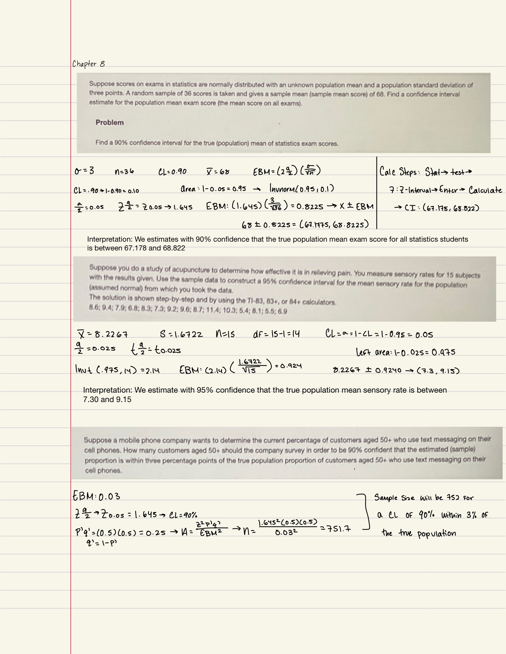
Examples