AP Econ Unit 3 (Microeconomics)

Topic 3.1 – The Production Function

Introduction to production functions

• A production function describes how inputs are used to produce outputs.
• Inputs in production functions are typically factors of production like land, labor, capital, and entrepreneurship. The short run-in production refers to a period where at least one input is fixed, while the long run is a period where none of the inputs are fixed.
• In the example of a bread-toasting operation, inputs include slices of bread, toasters, and workers.
• Production functions help analyze how different factors affect output in various economic scenarios.

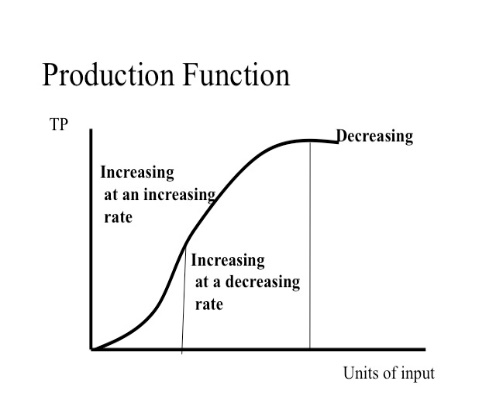
Total product, marginal product, and average product

• A production function takes inputs and generates output, and this video focuses on how output varies with a single input (labor).
• Total product (TP) is the amount of output produced as a function of labor. The ice cream factory example varies with the number of workers, e.g., 0 workers yield 0 gallons, 1 worker yield 10 gallons, 2 workers yield 18 gallons, and 3 workers yield 24 gallons.
• Marginal product of labor measures how much additional output is produced with the addition of one more unit of labor. It can be seen as the slope of the total product curve. For example, going from 0 to 1 worker adds 10 gallons, so the marginal product for that worker is 10.
• Diminishing marginal returns occur when adding more units of labor leads to a decreasing marginal product. This is because additional workers may become less productive due to various factors like waiting times or space constraints.
• A firm experiences increasing marginal product when its marginal costs are decreasing.
• Average product (AP) of labor is the total product divided by the number of workers. For instance, when there is 1 worker, the average product is 10 gallons (total product divided by 1 worker).
• One must increase the quantity of capital to avoid diminishing marginal returns to labor
  • Diminishing returns set in because more units of labor are using fixed amounts of other inputs, such as capital. If you add more workers to the same number of tools, diminishing returns set in, but if you add more workers and more tools, diminishing returns do not set in.

Topic 3.2 – Short-run Production Costs

Fixed, variable, and marginal costs

• The author is working on a software project and needs to determine the optimal number of programmers to hire for maximum productivity.
• Fixed costs in this scenario include office space and a product manager's salary, totaling $15,000 per month.

• Variable costs are the full compensation for a programmer, set at $10,000 per month per programmer.
• Total costs are calculated by summing fixed and variable costs.
• Average fixed costs per line of code decrease as more programmers are added to the project.
• Average variable costs per line of code increase as more programmers are added, reflecting diminishing productivity.
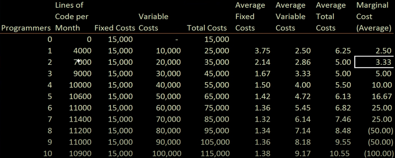• Marginal cost represents the incremental cost of producing additional lines of code, and it can become negative when too many programmers reduce overall productivity.

Marginal cost, average variable cost, and average total cost

• The video uses a hypothetical example of ABC Watch Factory to explain cost concepts in economics.
• Fixed costs are expenses that do not change in the short run, such as rent or equipment costs.
• Variable costs, which are influenced mainly by labor units and materials, change with the level of production.
• Total cost is the sum of fixed costs and variable costs.
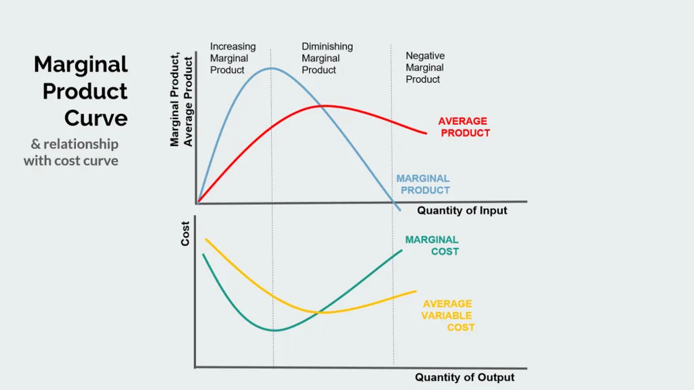
• Marginal product of labor measures how much additional output is produced when adding one more labor unit.
• MPL ($) = (Change in total cost) / (Change in total output)
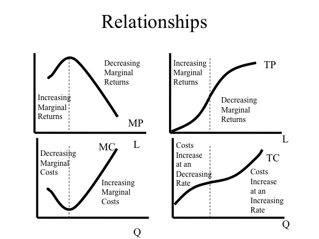• Initially, the marginal product of labor tends to increase due to specialization but later experiences diminishing returns.
• Marginal cost represents the cost of producing an additional unit of output.
• Marginal cost typically decreases initially as specialization leads to efficiency but later increases due to diminishing marginal returns.
• Average variable cost is calculated by dividing variable costs by total output.
• Average fixed costs are calculated by dividing fixed costs by total output.
• Average total cost is calculated by dividing total costs by total output.
• The video highlights that marginal cost intersects with average variable cost and average total cost, indicating a change in cost trends.

Graphs MC, AVC, and ATC

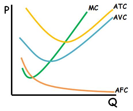• Marginal cost is plotted on the vertical axis (cost), and the horizontal axis represents the output.
• As output increases, marginal cost tends to rise, indicating diminishing returns.
• Average variable cost decreases initially as output increases but starts to rise when the marginal cost exceeds it.
• The intersection point of the marginal cost and average variable cost curves represents the minimum point of the average variable cost curve.
• Average total cost includes both variable and fixed costs and behaves similarly, but it intersects with marginal cost at a later point.
• The intersection of marginal cost and average total cost represents the minimum point of the average total cost curve.
• Average fixed cost decreases steadily with increased output due to spreading fixed costs over more units.
• When a firm’s only variable input is labor, the average variable cost (AVC) is lowest when the average product of labor is highest.

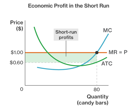
Marginal revenue, and marginal cost

• The market price for orange juice is 50 cents a gallon, and producers need to be price takers to remain competitive.
• Marginal revenue is constant at 50 cents per gallon when the market price is 50 cents.
• Producers aim to maximize production to spread their fixed costs over more gallons.
• The production quantity should not exceed the point where marginal cost exceeds marginal revenue.
• The rational amount to produce is when marginal revenue equals marginal cost, which is 9000 units in this scenario.
• Total revenue is calculated as the area under the marginal revenue line, and total cost is the area under the average total cost line.
• Profits are the difference between total revenue and total cost, which, in this case, results in a profit of $180.

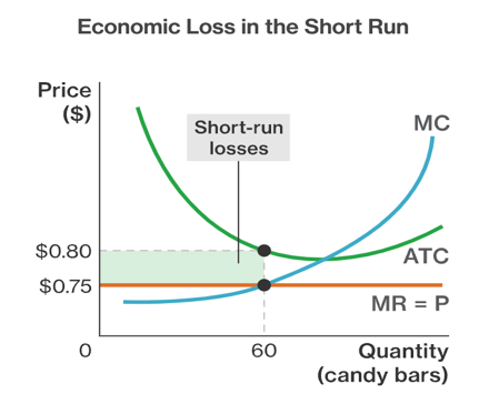
Marginal revenue below average total cost

• In microeconomics, it's essential to produce a quantity of a product that maximizes profit, considering the relationship between marginal cost and marginal revenue.
• The ideal production quantity is where marginal cost equals marginal revenue, which is equivalent to the market price in a competitive market.
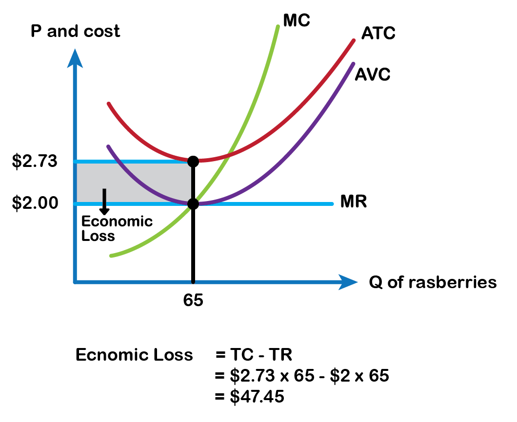• The video uses the example of producing 8,000 gallons of orange juice at a market price of $0.45 per gallon.
• At this quantity, marginal revenue is $0.45 per unit, but the average total cost is $0.48 per unit, resulting in a loss of $0.03 per unit or $240 for 8,000 gallons.
• Even though there's a loss, it may still make sense to produce some units to offset fixed costs.
• Continue to produce when MRDARP is greater than AVC!
• The fixed costs represent a committed expenditure and producing nothing would result in a weekly loss of $1,000.
• However, producing beyond the point where marginal cost exceeds marginal revenue would not be rational as it increases the loss.
• This short-term production strategy assumes fixed costs, but long-run decisions may involve adjusting costs and production quantities as fixed factors change.

How costs change when fixed and variable costs change

• When fixed costs increase, it does not affect the marginal product of labor, marginal costs, or average variable cost.
• Marginal product of labor depends on total output and labor units and is unaffected by fixed costs.
• Marginal costs are determined by changes in total costs divided by changes in output, and fixed costs do not impact on this calculation.
• Average variable costs are not affected by changes in fixed costs.
• Average fixed costs change when fixed costs change, as they are directly derived from fixed costs and output.
• Average total costs are based on total costs and are affected by fixed and variable cost changes.
• Labor productivity improvements can change the marginal product of labor, marginal costs, and average variable cost by altering total output for a given amount of labor.
• A productivity improvement increases output for the same labor input, impacting marginal costs and average variable costs.
• Changes in variable costs, such as wage increases, affect marginal costs and average variable costs, while fixed costs remain unaffected.

Graphical impact of cost changes on marginal and average costs

• Average fixed cost asymptotes toward zero as units increase, while the marginal cost curve is typically u-shaped.

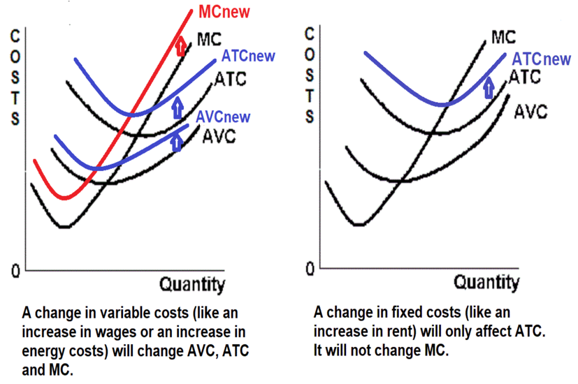
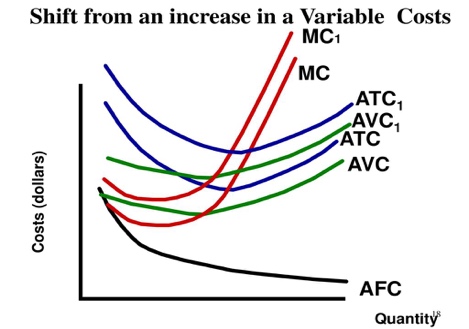
Change in Variable Costs

• Average variable cost intersects with marginal cost at its minimum point, causing average variable cost to shift from trending down to trending up.
• A similar trend occurs with average total cost as it intersects with marginal cost.
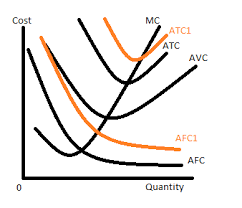• The difference between average total cost and average variable cost represents average fixed cost and tends to converge to zero over time.
• Changes in fixed costs, such as an increase in rent, would shift the average fixed cost curve upward, affecting average total cost as well.

Change in Fixed Costs

• Changes in variable costs, like a pay increase, shift the variable cost curve upward, impacting marginal cost.
• An increase in variable costs would likely result in higher incremental costs and affect the shape of the marginal cost curve.
• Changes in productivity affect average variable cost, marginal cost, and, by extension, average total cost. Changes in fixed costs only impact average fixed cost and average total cost.

Topic 3.3 – Long-run Production Costs

Long-run average total cost curve

• Average total cost is the sum of average variable cost and average fixed cost.
• Short run refers to a period during which at least one input is fixed, while the long run allows for adjustments to all inputs.
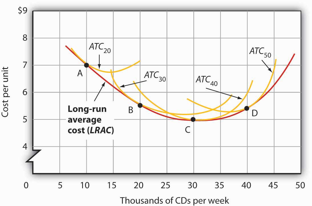• To optimize fixed costs for a specific quantity (e.g., 200 tacos per day), you may need to adjust the number of food trucks.
• Short-run average total cost is illustrated as a curve with fixed inputs (e.g., two food trucks), and its shape changes based on actual demand.
• Long-run average total cost is a curve connecting the minimum points of various short-run curves, representing the optimal cost for different production quantities.
• In the long run, businesses can choose the ideal number of trucks for each level of demand, resulting in cost efficiency.

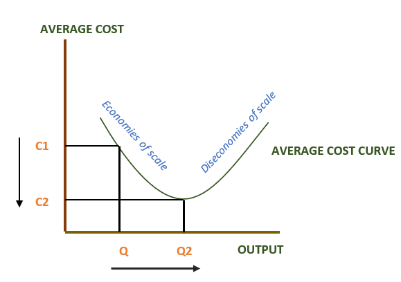
Economies and diseconomies of scale

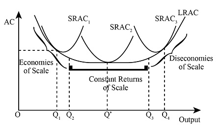• Economies of scale occur as a company becomes more efficient in producing goods as it increases production quantities.
• Specialization of labor and sourcing, as well as potential cost savings, can lead to economies of scale.
• Diseconomies of scale result from coordination issues and the increasing complexity of managing larger organizations.
• Depletion of resources, higher labor costs, and coordination challenges are common causes of diseconomies of scale.

EOS: Specialization & Cost Savings

DOS: Depletion of Resources, Higher Labor Costs, & Coordination Challenges

• The concept of constant returns to scale represents a phase where long-run average total costs neither increase nor decrease significantly.

Minimum efficient scale and market concentration

• Minimum efficient scale (MES) is the point at which economies of scale cease, and the long-run average total cost curve no longer declines.
• MES is essential for a firm to be competitive and efficient in the market.
• MES can vary based on the industry and the specific market conditions.
• In a competitive market, firms operating at MES can remain profitable even with lower prices, while those below MES may struggle.
• The higher a firm’s fixed costs, the higher a firm’s minimum efficient scale it will have.
• Market size varies depending on how the market is defined, such as the market for tacos in a city.
• When MES is a small fraction of the total market, it leads to a fragmented market with numerous competitors.
• When MES is close to or larger than the market size, it results in a concentrated market, potentially leading to a natural monopoly.

Topic 3.4 – Types of Profit

Economic profit vs. accounting profit

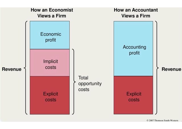• The text explores the distinction between accounting profit and economic profit in the context of a restaurant business.
• Goal: Maximize economic profit
• Accounting profit represents the traditional way of calculating profit, where revenue is subtracted from explicit expenses to determine profit.
• Economic profit considers opportunity costs, including both explicit and implicit costs.
• Explicit opportunity costs are direct outlays of the business, measured in dollars, while implicit opportunity costs are the foregone earnings or benefits due to the chosen business activity.
• Economic profit can be negative, indicating that it might not make sense to continue the business in its current form, as the owner could potentially earn more elsewhere.
• EP = (P-ATC) x Q
• AP = (P-AEC) x Q
• To ensure that a firm is earning an economic profit, the price of the good must be higher that the firm’s average total cost
• The calculation of economic profit helps decision-makers assess whether a business is the most profitable option and whether they should consider alternative opportunities.

Topic 3.5 – Profit Maximization

Profit maximization

• Profit in a firm is determined by subtracting its costs from its revenue, and rational firms aim to maximize their profit.
• To achieve profit maximization, firms need to consider the relationship between marginal cost and marginal revenue.
• In a competitive market, a firm is a price-taker, meaning that the incremental revenue per unit produced remains constant.
• If the marginal revenue is higher than the marginal cost, it is rational for the firm to keep producing more units. (MR = MC)
• The point at which marginal cost equals marginal revenue is where a firm should stop production to maximize profit.
• The area between the marginal cost and marginal revenue curves represents the profit a rational firm can make.
• Producing fewer or more units than the profit-maximizing quantity results in lower profits due to a loss on incremental units with higher marginal costs.

Profit maximization worked example

• The scenario involves corn production in a perfectly competitive market, used for food and ethanol.
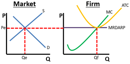• Two side-by-side graphs are created: one for the corn market and one for a representative corn farmer.
• The equilibrium price and quantity in the corn market are denoted as P sub-M and Q sub-M, respectively.
• The farmer's profit-maximizing quantity (Q sub-F) is calculated, with the constraint of zero economic profit.
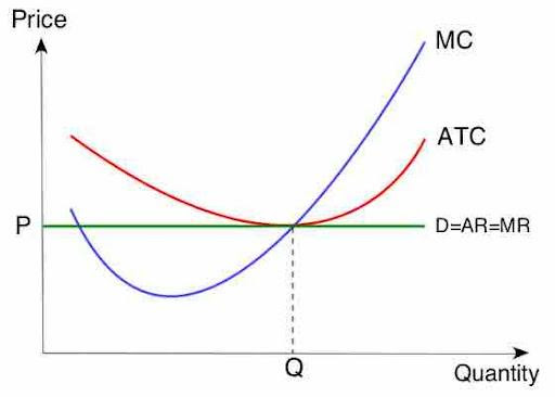
• In a perfectly competitive market, the farmer is a price taker, and their marginal revenue equals the market price.
• The farmer's profit-maximizing quantity is where marginal cost intersects marginal revenue (market price), with the price equal to the average total cost.
• The point of intersection of marginal cost and average total cost corresponds to the profit-maximizing quantity (Q sub-F).

Topic 3.6 – Firms’ Short-run Decisions to Produce and Long-run Decisions to Enter or Exit a Market

Shutting down or exiting industry based on price

• In a perfectly competitive market, a firm is a price-taker and produces where marginal cost equals marginal revenue.
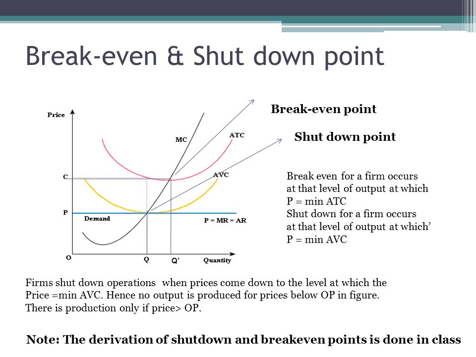• When the market price is higher than the average total cost, the firm is profitable and likely attracts new entrants.
• If the market price equals the average total cost, the firm operates at a break-even point and doesn't attract new entrants.
• When the market price falls below the average total cost but remains higher than the average variable cost, the firm operates in the short-run but exits in the long-run.
• If the market price falls below both the average total cost and the average variable cost, the firm shuts down in the short-run and exits in the long-run.
• IF THE MARGINAL REVENUE (PRICE) IS BELOW ATC, THEN IN THE LONG-RUN, EXIT THE MARKET
• EXITING THE INDUSTRY IS A LONG-RUN BEHAVIOR! – NOT SHORT-RUN

Topic 3.7 – Perfect Competition

Introduction to perfect competition

• Perfect competition in microeconomics involves many buyers and sellers offering identical products or services.
• Participants in perfect competition have perfect information, meaning they know what is happening in the market, including prices and transactions.
• The concept of no barriers to entry or exit in perfect competition is idealized and rarely exists in the real world.
• In a perfectly competitive market, firms are passive price takers and have no control over the market price.
• Firms in perfect competition produce where their marginal cost intersects with their marginal revenue to maximize profit.
• The passivity of firms in perfect competition contrasts with the idea of fierce competition where firms constantly undercut each other.
• Perfect competition may not be desirable in certain industries like healthcare, where barriers to entry ensure a certain level of training and expertise.

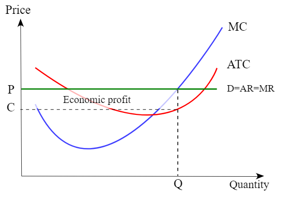
Economic profit for firms in perfectly competitive markets

• Market Power is the firm’s ability to control the price of a good.
• Market supply and demand curves define the price, and firms must accept this price for their products.
• Firms aim to produce the quantity where marginal cost equals marginal revenue (equal to the market price).
• Economic profit is calculated as the area between the price (marginal revenue) and average total cost multiplied by the quantity produced.
• Firms will only produce quantities where marginal cost is less than or equal to the market price.
• In a perfectly competitive market, a firm makes a profit if the area between price and average total cost is positive.
• Economic losses occur when the area between price and average total cost is negative.
• In the short run, firms have fixed costs, but in the long run, they can choose to enter or exit the market based on their profit or loss situation.
• Firms with economic losses may exit the market in the long run if they cannot cover their fixed costs.

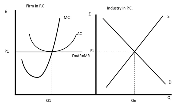
Long-run economic profit for perfectly competitive firms

• In perfectly competitive markets, firms are price takers, and their marginal revenue curve is horizontal, equal to the market price.
• Firms aim to produce if marginal revenue is higher than marginal cost to maximize profit in the short run.
• Economic profit is the difference between the price and average total cost, representing profit per unit multiplied by the number of units produced.
• In the long run, new firms enter the market when they see others making economic profit, causing the supply curve to shift to the right.
• As more firms enter, the market price decreases, and each firm's marginal revenue curve changes.
• Firms adjust their production quantities in response to changing market conditions and the new equilibrium price.
• As more entrants join, economic profit decreases until it reaches zero, and firms become productively efficient.
• Productive efficiency is achieved when firms produce at the minimum point of the average total cost curve.
• Allocative efficiency is also maintained in the long run as the market equilibrium ensures marginal benefit equals marginal cost.
• In some cases where too many firms enter the market, economic losses may occur, leading some firms to exit and shifting the supply curve to the left.
• Short run: allocatively efficient; Long run: allocatively efficient and productively efficient

Long-run supply curve in constant const perfectly competitive markets

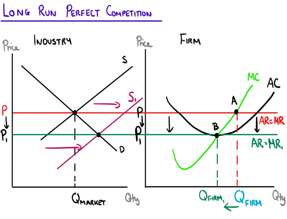
• In a perfectly competitive market in the long run, firms operate at zero economic profit, as they are price takers with a horizontal marginal revenue curve.
• Economic profit accounts for opportunity costs and may differ from accounting profit.
• If market demand increases in the short run, the demand curve shifts to the right, leading to higher equilibrium prices and quantities.
• Firms in the market, like Firm A, can experience economic profit in the short run due to increased demand.
• In the long run, new firms will enter the market since there are no barriers to entry, and this will cause the supply curve to shift to the right.
• In a constant cost, perfectly competitive market, the entering or exiting of firms does not affect the cost structures of the firms.
• The long run supply curve in a constant cost, perfectly competitive market is a horizontal line, indicating that firms can produce any quantity at the same cost.

Long-run supply when industry costs aren’t constant

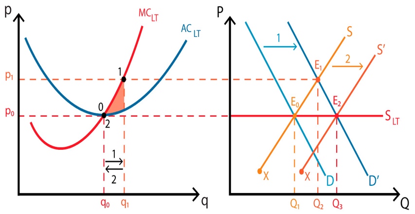
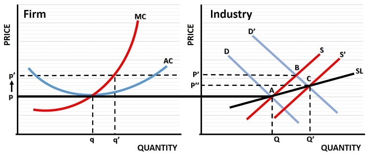• In a perfectly competitive market, the equilibrium price is determined by the intersection of supply and demand curves.
• Rational quantity for a firm to produce is where marginal revenue intersects marginal cost, leading to zero economic profit.
• Positive economic profit attracts more firms to enter the market, while negative profit leads to exits.
• A shock in the market, such as increased demand for a product like apples, can lead to a new equilibrium price and quantity.
• When more firms enter a market with positive economic profit, input costs may rise, changing the cost structure.
• Changing cost structures result in a new marginal cost curve and average total cost curve.
• Economic profit for all firms goes to zero when marginal revenue equals marginal cost and average total cost.
• Long-run supply curves in an increasing cost market shift to the right as more firms enter, leading to higher equilibrium prices.
• Long-run supply curves can be upward-sloping in an increasing cost market and downward-sloping in a decreasing cost market.
• If the market for tacos is a perfectly competitive decreasing cost industry, an increase in demand decreases prices in the long-run.