9. Introduction to t-statistics

Introduction to t-statistics, Independent and Related Sample t-test

The t Statistic: An Alternative to z

• Z-score: A statistical procedure testing hypotheses about an about an unknown population average/mean using the average/mean from a sample

• Basic Concepts:

  • Sample Mean (M) can be use to determind the approximate of Population Mean (μ).

  • Standard Error: Measures how well a sample mean approximates the population mean.

  • Compare sample mean (M) with hypothesized population mean (μ) with z-score calculation.

The Problem with z-Scores

• Goal: Determine if the difference between data and hypothesis is significant.

• Z-scores require knowledge of the population's standard deviation, which is often unknown.

• Using sample standard deviation instead of population standard deviation allows hypothesis testing to proceed

Introduction to t-statistics

• Estimated Standard Error (sM): Used as an estimate of the real standard error (σM) when population standard deviation(σ) is unknown, derived from sample variance or standard deviation.

t-statistic Formula

• t-statistics/t-value:how far your sample mean is from the population mean, adjusted for the size and variability of your sample.

• Usage: Tests hypotheses about an unknown population mean (μ) when population standard deviation(σ) is unknown.

• Formula structure is similar to z-score but uses estimated standard error in the denominator.

  

• Types:used in different contexts depending on what you're comparing;

  1. One-sample t-test (comparing a sample mean to a population mean)=

     • testing a hypothesis about an unknown population mean (μ)

     • formula:calculate the t-value by comparing the sample mean to the hypothesized population mean, adjusting for the sample size and variability (sample standard deviation)

       

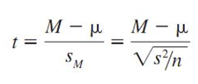
       M =sample mean which represents the average of the sample data.

       𝜇 =population mean (the hypothesized mean you are testing against)

       𝑆 =sample standard deviation, which is used to estimate the population standard deviation.

       𝑛 =sample size.

       𝑆𝑚 =standard error of the mean, It represents the variability of the sample mean.

       *Since you don't know the population's standard deviation, you use the sample's standard deviation to calculate the t-value.

     (Two-sample t-test Isn’t in the ppt so it isn’t as important, focus on One-sample t-test)

  2. Two-sample t-test (comparing two sample means)=

     • comparing means of two samples from different population, often when you want to determine if the two groups come from populations with different means.

     • formula:measures how far apart the sample means are, adjusted for the variability within each sample and their sizes, difference between the two sample means is statistically significant.

       

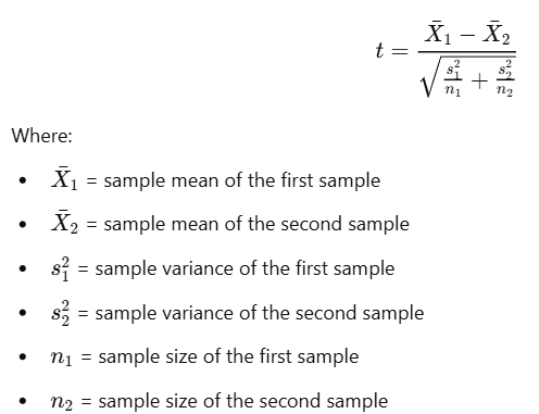
       *don't know the population standard deviations, you use the two-sample t-test

• Degrees of Freedom (df): counting how many numbers in a set are "free to move" or change without messing up the average

  *for sample, not population

  • first two numbers could vary, but the last number is locked in once the first two are chosen for the average to be the same;

    *ex= Imagine you have 3 numbers that must add up to 10. Let’s say:

    The first number is 3.

    The second number is 4.

    Now, the third number must be 3 (because 3+4+3=10)

  • mean depends on the total. That’s why the formula is:

    Degrees of Freedom (df)=n(total number of values in the sample)−1

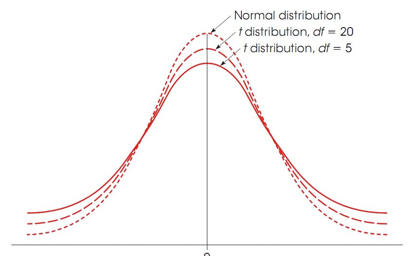
The t Distributions

• The t distribution=a curve(not a formula) that shows the probability of getting a certain t-value/something more extreme if the null hypothesis is true, based on small samples.

  • It’s like a normal distribution, but you use it when you don’t know the population standard deviation or working with fewer data points.

• t-distribution collects all these t-values to show how they behave for a specific sample size or degrees of freedom

• Shape/Curve=

  • looks like the normal distribution (a bell curve), but it’s a bit wider, especially with smaller sample sizes.

  • sample size gets bigger, the t-distribution becomes nearly identical to the normal distribution.

    

• Types of Tail:

  1. Proportion in One Tail

     • A "tail" is the far left or far right end of the curve(probability in one end of the distribution)

     • probability of tail=

       1. Proportion in one tail = 0.05 or 5% → This is the amount of extreme on one side (0.05 or 5%)

  2. Proportions in Two Tails Combined:

     • combined probability in both tails(left and right)

       *interested in extreme values at both ends of the curve (very low or very high t-values) because either could show that the null hypothesis is unlikely.

     • probability of tail=

       1. Two tails combined= Left tail + Right tail

       2. proportion of individual tail= Left tail + Right tail

          —————————-

          2

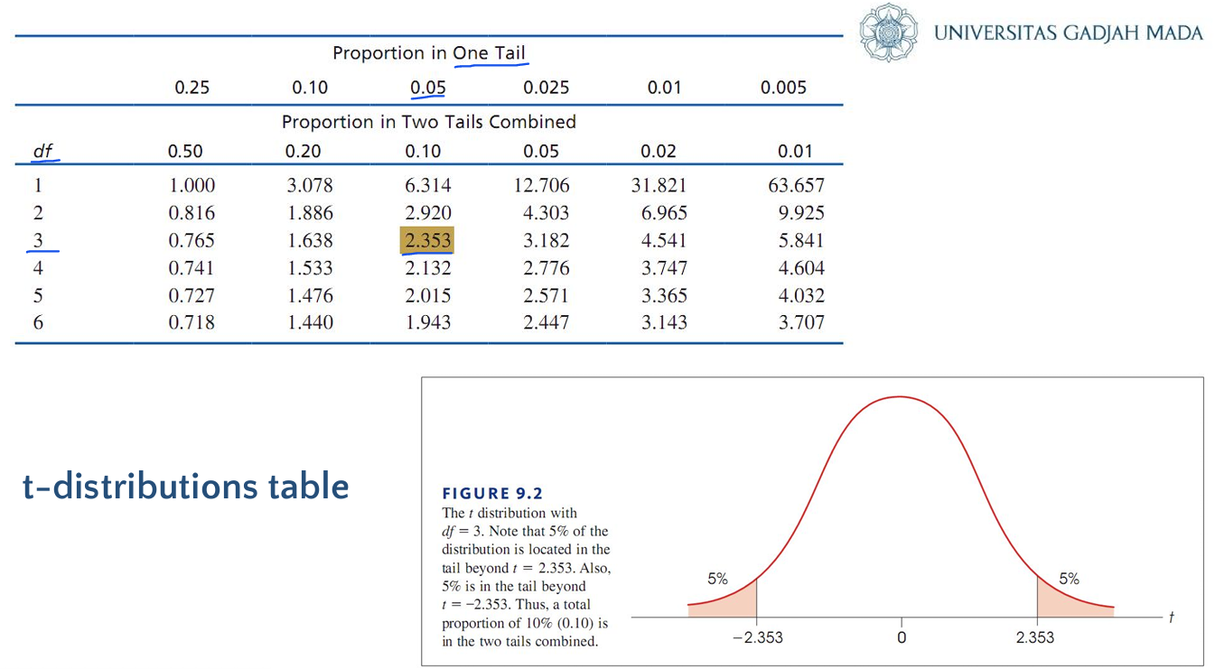
Determining Proportions and Probabilities for t Distributions (t-distributions Table)

Use a t-distribution table to find proportions for t statistics.

• t-Distribution Table: A table that give a specific number of;

  • A t-value if you know the probability.

  • A probability if you know the t-value.

  if the null hypothesis is true, based on small samples

  *shortcut for getting t-value/probability

• How to read the question:

  • One tail/two tails combined=

    1. One tail

       • “tail beyond” refers one end of the distribution, either the far right or far left.

         “Tail beyond t = 2.353 occupies 5% of the distribution”

         -with the number/probability occupied refers specifically to the area in one tail, not the total area in both tails

         (5% one tail)

    2. Two tails combined

       • "Combined tails beyond” refers to the combined distribution

         “Combined tails beyond ±2.353 occupy 5% of the distribution”

         -with the number/probability occupied refers to two tails combined (2.5% in each tail)

  • direction of the tail=

    1. Positive/negative

       • Right tail(higher values on the curve)

         - t-value = positive (e.g.,t=2.353)

       • Left tail(lower values on the curve)

         - t-value = negative (e.g.,t=−2.353)

    2. Key words

       • Right tail

         -question says "beyond" t = 2.353, because it’s looking at values greater than t=2.353

       • Left tail

         -question says "below" or "less than" t = -2.353, because it’s looking at values smaller than t=−2.353

    3. Context of the problem

       • Right tail

         -problem involves testing whether values are greater than the mean

       • Left tail

         -problem involves testing whether values are less than the mean

• Problem example:

  • df = 3(this comes from your sample size minus 1)

    Tail beyond t = 2.353 occupies 5% of the distribution

    ↓ ↓

  “Tail beyond”=one tail positive number=right tail

• Process:

  1. Step 1: Look up the degrees of freedom (df) in the table (in this case, 3).

  2. Step 2: Find the desired probability (in this case, 0.05, or 5%).

  3. Step 3: The table will show you the t-value that corresponds to that probability. For df = 3 and 5%, the t-value is 2.353.

     

Independent and Related Measure Designs

• Between-Subjects Design(Independent Measures Design):

  • A research design that uses a separate group of participants for each treatment condition

  • goal= compare the effects of each conditions on the two groups

  • The Hypotheses for independent measure=

    H0: µ1 − µ2 = 0

    H1: µ1 − µ2 ≠ 0

  • formula=

    

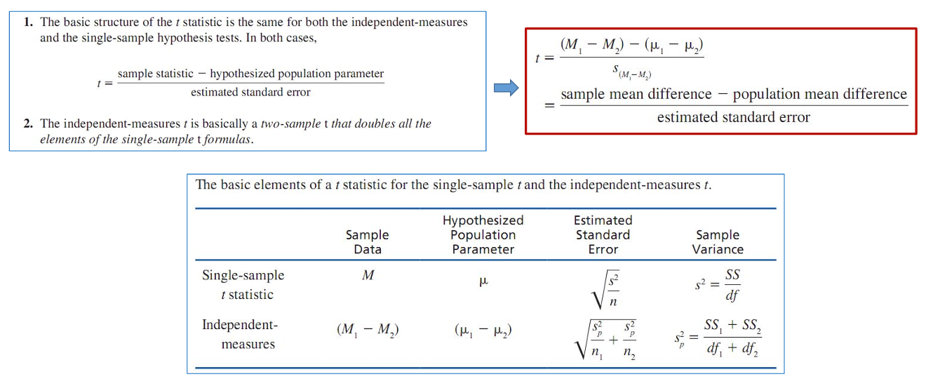
  • Independent Sample t-test Calculation:

    • used to compare the averages (means) of two different groups.

    • steps=

      1. State hypotheses and alpha level:

         -Hypotheses=make a claim about Null hypothesis (H₀) & Alternative hypothesis (H₁)

         -Alpha level=cut-off value, helps decide if your results are statistically significant

      2. Determine degrees of freedom (df) and critical region using the t-distribution table:

         -determine the degrees of freedom (df)

         -Critical region=reject the null hypothesis if your t-statistic falls in this region

      3. Compute the test statistic (t-statistic):

         -calculate using Two-sample t-test

      4. Compare t-statistic with critical values to make a decision:

         -compare t-statistic to the critical t-value you found in the t-table;

         • If the t-statistic is greater than the critical t-value, you reject the null hypothesis(there is a significant difference between the two groups)

         • If the t-statistic is smaller, you fail to reject the null hypothesis (there’s no significant difference)

• Within-Subjects Design(Related Measures Design):

  • A research design that uses the same group of participants which experience all treatments.

    *test the same individuals more than once, with each person going through every condition or treatment

  • goal: comparing their performance in two different conditions, but each person is tested with both conditions.

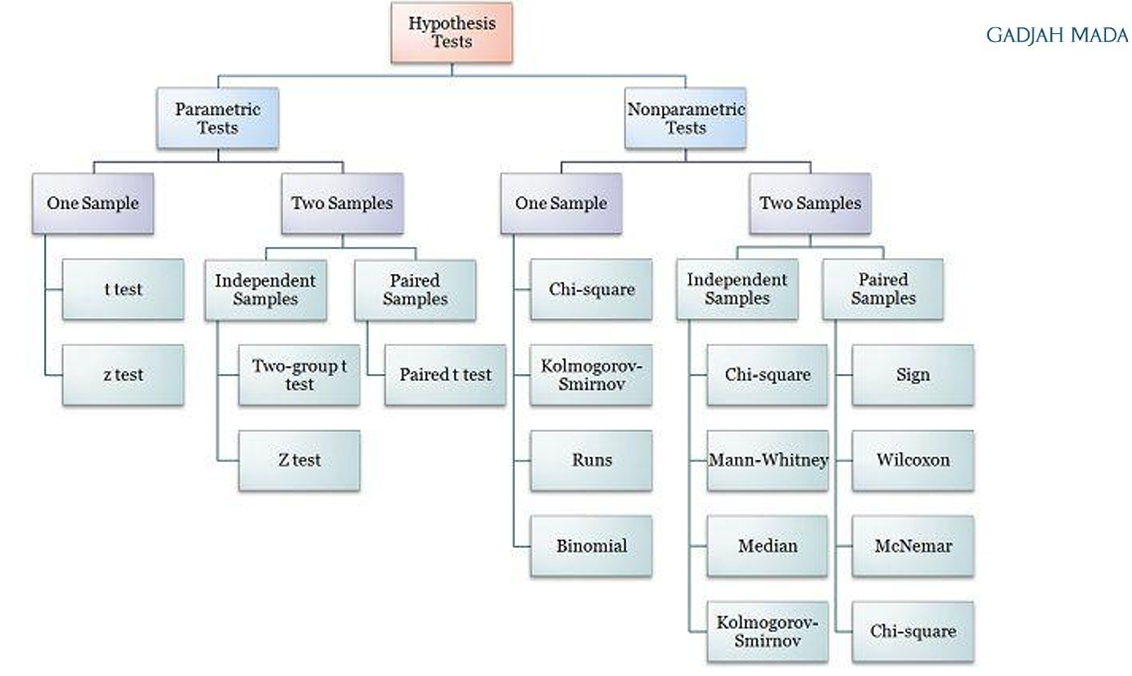
Parametric vs Nonparametric Statistics

• Parametric Statistics: way of analyzing data where you make assumptions about how the data behaves in the population;

  *such as following a specific pattern or distribution(like assuming it follows a normal distribution; bell-shaped curve)

  • key assumptions=

    1. Additivity= assumes that the impact of one factor is independent of the impact of the other factors, so you can just sum them up to get the total effect

    2. Normality= data should follow a normal distribution (a bell-shaped curve)

    3. Homogeneity of Variance= The spread or variability of data should be the same across groups.

    4. Independence: Each data point should be independent of the others (one person’s result doesn’t affect another’s)

• Nonparametric Statistics: Way of analyzing data with no assumptions about the distribution at all

Hypothesis Tests

Example - Independent Sample t-test

• Describes an experiment testing the effect of lighting on puzzle-solving performance and the resulting potential for cheating.

Example Step - Hypothesis and Alpha Level

• Alpha level set at 0.05. Directional hypotheses may specify expected outcomes based on environmental conditions.

Example Step - Compute Test Statistic

• Analyzed significance of t value (-2.67) indicating a substantial difference in performance based on environmental lighting.

Calculating Effect Size: Cohen’s d

• Effect size measurement standardizing mean difference between two groups, reported as Cohen's d.

Repeated Measure Test

• Describes within-subject designs measuring dependent variables multiple times.

• Matched-Subjects Design: Individuals matched across samples based on specific variables.

Related Sample t-test

• t statistic is derived from difference scores rather than raw data, with hypotheses:

  • H0: µD = 0

  • H1: µD ≠ 0

Related Sample t-test Visualization

• Illustration of how each individual is measured twice with computation of difference scores.

Related Sample t-test Calculation Steps

• Similar to independent measures but includes obtaining data from related measurements.

t-test Summary

• Comparison of scores between independent and related samples, including considerations for bias and assumptions.