AP Precalculus- Unit 2: Exponential and Logarithmic Functions Flashcards
Arithmetic and Geometric Sequences
Sequence: an ordered list of numbers, with each listed number being a term. It could be finite or infinite

Arithmetic Sequence: when each successive term in a sequence has a common difference (constant rate of change)
Geometric Sequence: when each successive term in a sequence has a common ratio (consistent proportional change)
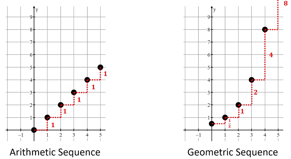
Over equal-length input-value intervals, if the output values of a function change:
at a constant rate → linear function (addition)
at a proportional rate → exponential function (multiplication)
^ all can be determined by two distinct sequence or function values
nth term (arithmetic): an = a0 + dn a0 = initial value (zero term) d = common difference (similar to slope-intercept form) |
nth term using any term (arithmetic): an = ak + d (n – k) ak = kth term of the sequence (similar to point-slope form) |
nth term (geometric): gn = g0rn g0 = initial value (zero term) r = common ratio (similar to exponential function) |
nth term using any term (geometric): gn = gk ∙ r(n – k) gk = kth term of the sequence (similar to shifted exponential) |
Exponential Functions f(x) = bx
-are always increasing or always decreasing
└ no extrema except on a closed interval
-always concave up or always concave down
└ no inflection points
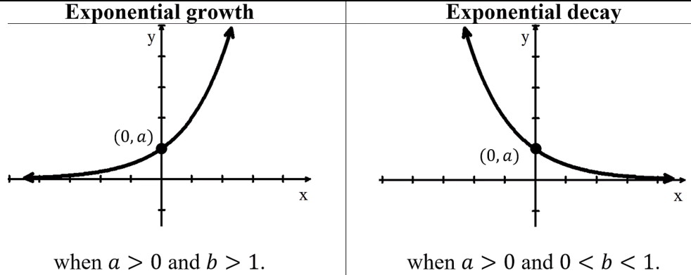
-if input values increase/decrease without bound, end behavior:
 or
or
 or
or

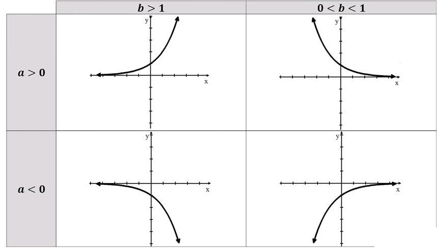
Horizontal Translation/Vertical Dialation: f(x) = b(x+k) = bx ∙ bk = abx where a = bk
Horizontal Dialation: f(x) = b(cx) → change of the base of function bc is a constant and c ≠ 0
Exponential functions model growth patterns with successive output values over equal-length input-values intervals are proportional
A constant may need to be added to the dependent variables of a data set to see proportional growth pattern
An exponential function can be constructed from: a ratio and initial value/two input-output pairs
base of exponent (b) → growth factor in successive unite changes in input values; percent change in context
forms of exponential functions can be used in different scenarios:
ex. if d = number of days f(x) = 2d → quantity increases by factor of 2 every day
f(x) = (27)(d/7) → quantity increase by a factor of 27 every 7 days/week
General Form of an Exponential Function: An exponential function has the general form f(x) = abx a = initial value ≠ 0 b > 0 |
Additive Transformation of an Exponential Function: g(x) = f(x) + k If the output values of g are proportional over equal-length input-value intervals, then f(x) is exponential |
Negative Exponent Property: b-n = (1/bn) |
Product Property: bmbn = b(m+n) |
Power Property: (bm)n = bmn |
The number e: e = 2.718… the natural base e is often used as the base in exponential functions |
Competing Function Model Validation
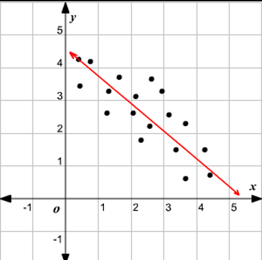
Model can be an appropriation for data if data set/regression is without pattern
Predicted vs actual results → error in model
May be appropriate to overestimate/underestimate for given interval
Composition of Functions
(f ⸰ g)(x)/f(g(x)) à maps set of input values to set of output values such that the output values of g are used as input values of f
└ domain of composite function is restricted to input values of f for which the corresponding output values is the domain of f
Typically, f(g(x)) and g(f(x)) are different values as f ⸰ g and g ⸰ f are different functions
Additive Transformations → vertical/horizontal translations (g(x) = x + k)
Multiplicative Transformations → vertical/horizontal dilations (g(x) = kx)
Identity Function:
when f(x) = x
Then g(f(x)) = f(g(x)) = g(x)
Acts as 0 (additive identity) when adding
Acts as 1 (multiplicative identity) when multiplying
Inverse Functions
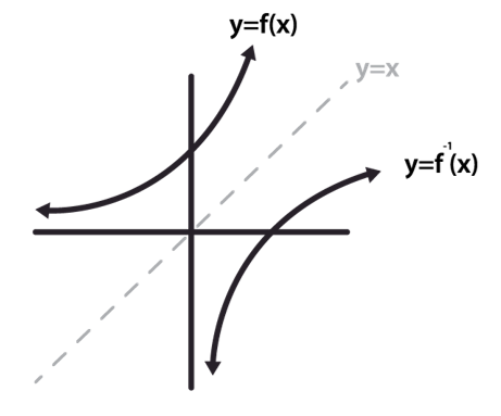
Inverse Function → in each output value is mapped from a unique input value
Ex. f(x): inputs on x-axis and outputs on y-axis (f(a) = b) →
f-1(x): inputs on y axis and outputs on x axis (f-1(b) = a)
composite of function and inverse = identity function
 function’s domain and range → inverse function’s range and domain (respectively)
*domain may be restricted
Inverse of Exponential Functions
f(x) = a logb x with base b, where b > 0, b ≠ 1, and a ≠ 0
generally, exponential functions and log functions are inverse functions (reflections over h(x) = x)
└ f(x) = logb x and g(x) = bx → f (g(x)) = g( f(x)) = x
exponential growth → output values changing multiplicatively as input values change additively
logarithmic growth → output values changing additively as input values change multiplicative
Logarithmic Functions
logbc = value b must be exponentially raised to in oder to obtain the value c
logbc if and only if ba = c (a & c = constants) (b > 0) (b ≠ 1)
if b not specified, log is common log with base 10 (b = 10)
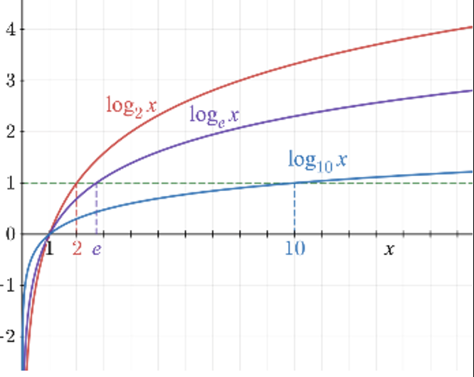
used to model situations involving proportional growth or repeated multiplication
a logarithmic function can be constructed from a proportion and a real zero/ two input-output pairs
each unit represents a multiplicative change of the base of the log
domain of general form → any real number greater than 0
range of general form → all real numbers
If input values of the additive transformation function g(x) = f (x + k) are proportional over equal-length output value intervals à →(x) is logarithmic (Does not apply vice versa)
since inverse of exponential function → logarithmic functions are:
- always increasing or always decreasing
- always concave up or always concave down
- do not have extrema except on closed intervals
- do not have points of inflection
In general form, features of log function include:
-vertically asymptotic to x = 0
-end behavior is unbounded
└ or
or

Log Product Property:
|
Log Quotient Property:
|
Log Exponential Property:
|
Natural Log Property:
|
Exponential and Logarithmic Equations and Inequalities
- must look for extraneous solutions
-exponential can be written as log functions
 combination of transformations of exponential function in general form *
 combination of transformation of log function in general form *
* inverse of function can be found by determining the inverse operation to reverse the mapping
Semi-Log Plots
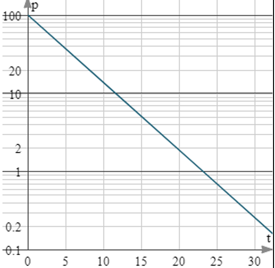
- y-axis is logarithmically scaled, while the x-axis is linearly scaled
- used to visualize exponential functions
- a constant does not need to be added to reveal that an exponential model is appropriate
- linear model for semi-log plot:
 where n > 0 and n ≠ 0
└ linear rate of change: 
└ initial linear value:

 Knowt
Knowt


