ECON 2105 Final

Economics Lecture 1, Unit 1 January 8 Notes:

• There are several differing definitions for economics, scarcity being the heart of all these definitions.
• Examples: “Economics is the study of how society a manages its scarce resources.” Greg Mankiw and “Economics is the science which studies human behaviour as a

relationship between ends and scarce means which have alternative uses.” Lionel Robbins

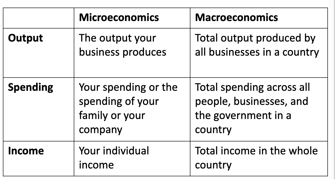
• Microeconomics is the study of choices that individuals and businesses make, the way those choices interact in markets, and the influence of specific government policies.
• Macroeconomics is the study of performance of whole national or global economies.

Chapter 1: Ten Big Ideas Notes-

1. Incentives Matter

• Incentives-rewards and penalties that motivate behavior.
• Ex. Journey to private contractors that would take convicts to Australia. There were mistakes in this planning because it paid for convicts getting to Australia but not off in Australia, so the convicts did not have as much food and medicine as they needed.
• People respond to all kinds of incentives in predictable ways

- Subsidies vs taxes: Putting subsidies on cars, or taxes on things which lead to people buying less of it.

• Incentives do not just have to be monetary. People are not only interested in money but pride, and being likeable.
• Incentives need not be monetary.

- Fame, power, reputation, etc are all important incentives.

1. Good Institutions Align Self-Interest with the Social Interest

• When markets work well, individuals pursuing their own interest also promote the social interest as if led by an “invisible hand”
• When markets do not work well, government can change incentives with taxes, subsidies, or regulation.

1. Trade-Offs are Everywhere

• Trade-offs involved for drug testing
• In our world of scarcity, all choices come with opportunity costs.

- A resource is scarce when there isnt enough to satisfy all of our wants

- The opportunity cost of a choice is the value of the opportunities lost, namely the value of the next best alternative you must give up when making a choice.

• Every choice involves something gained and something lost.
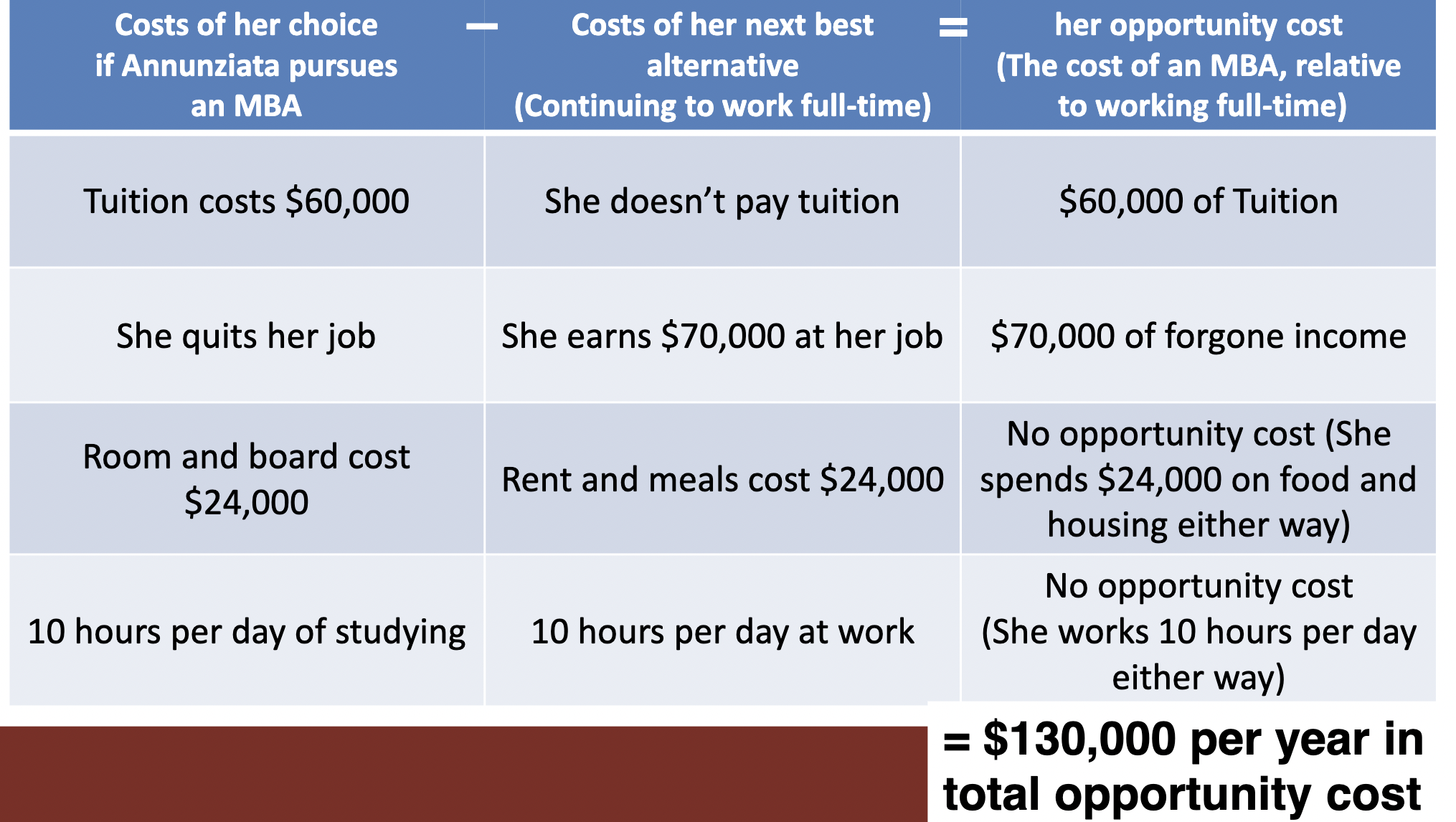
• How would we quantify the opportunity cost of Annunziata pursuing a two-year MBA full time?

- She pays $60,000 in tuition, pays for room and board, spends time studying, and quits her current job (loses that income)

Compared to what happens if she pursues her next best alternative:

- She earns $70,000 per year, still has to pay rent, and meals, and spends her time working.

Four Important Lessons About Opportunity Costs:

1. Some out-of-pocket costs are opportunity costs, such as the cost of MBA tuition and fees.
2. Opportunity costs don’t need to involve out-of-pocket financial costs.
3. Not all out-of-pocket costs are real opportunity costs.
4. Some nonfinancial costs are not opportunity costs.

When ignoring opportunity costs, you should ignore sunk costs.

• A sunk cost is a cost that has been incurred and cannot be reversed.
• A sunk cost exists whether you make your choice or not, so it is not an opportunity cost.
• When weighing costs and benefits, a good decision maker ignores sunk costs.

4. Think on the Margin

• We make choices by comparing marginal costs and marginal benefits.

- Marginal means one unit more or fewer, so a marginal cost is the cost of consuming one more unit of a good and the marginal benefit is the benefit from consuming that unit.

• Rational people will only pursue choices where the marginal benefit is greater than or equal to the marginal cost.

Applying the Cost-Benefit Principle-an example:

• How do we compare intangible benefits to monetary costs?
• Economists’ strategy: Convert each cost and each benefit into its monetary equivalent.

- What is your willingness to pay?

- That is, what is the most you would be willing to pay to obtain a particular benefit or avoid a particular cost?

• Ex. Are you willing to pay $7 for a coffee? How about $5? Or $3 or $1?
• The amount you are willing to pay depends on how much you like coffee, not the price.
• Suppose you are a bit tired and willing to pay up to $4 for a coffee
• Cost-benefit principle:
• The cost of the coffee=$3
• The benefit of the coffee=$4
• The benefit is greater than the cost.

After getting that coffee, you wouldn’t likely benefit from a second coffee as much as the first coffee. The marginal benefit of a second cup would thus be lower than the marginal cost, so you wouldn’t buy it.

• Barring violent compulsion, people wouldn’t participate in an exchange unless its marginal benefit to them exceeded its marginal costs.
• But the benefits of trade go beyond the benefits from exchange.

- Trade leads to increased production through specialization

- It also allows us to take advantage of economies of scale.

Theory of Comparitive Advantage:

• When people or nations specialize in goods in which they have a low opportunity cost, they can trade to mutual advantage

6. Wealth and Economic Growthh Are Important

• Economic growth creates wealth.
• Wealthier economies enable richer and healthier lives.

7. Institutions Matter

• Remember Principle 2: “Good Institutions Align Self-Interest with the Social Interest”

- On a broader scale, good institutions also provide incentives to save and invest in:

- Physical capital

- Human capital

- Innovation

- Efficient organization

• The right institutions foster growth:

- Property rights

- Political stability

- Honest government

- Dependable legal system

- Competitive and open markets

8. Booms and Busts Cannot be Avoided But Can be Moderated

• Economies do not grow at a constant pace.
• Booms and busts are a normal response to changing economic conditions
• In a downturn, output (GDP) drops and unemployment increases.
• The government can use fiscal and monetary policy to reduce the swings in output and unemployment.
• If used improperly, these tools can make the economy more volatile.

9. Inflation is Caused by Increases in the Supply of Money

• Inflation-An increase in the general level of prices.
• A country’s central bank regulates the supply of money.
• A sustained increased in the supply of money, without an increase in the supply of goods, causes prices to rise.
• Inflation can make people poorer.
• Unpredictable inflation makes it harder for people to figure out the real values of goods, services, and investments.
• Excessive inflation can lead to economic disruption.

10. Central Banking is a Hard Job

• The U.S. Federal Reserve (“the Fed”) is often called on to combat recessions.
• There are lags between a decision by the Fed and the effects of the decision
• In the meantime, economic conditions may change-they are a “moving target”.
• Too much money leads to inflation
• Not enough money can lead to economic slowdown or recession.

Takeaways:

• Understanding incentives matter, because people pursue their self-interest in the context of their institutional environment.
• This involves looking at the marginal benefits and costs as people face tradeoffs in a world of scarcity.
• These basic principles apply across countries, making it important that policymakers have a good understanding of their applications.
• Economics is also linked to everyday life-your job, personal finances, debt, inflation, recession.

Chapter 2: The Power of Trade and Comparitive Advantage

Introduction:

Benefits of Trade:

1. Trade makes people better off when preferences differ
2. Trade increases productivity through specialization and the division of knowledge
3. Trade increases productivity through comparative advantage

Trade and Preferences:

• Ex. Creator of ebay put up a random object, a broken pen as a way to try out the website, and actually got a buyer who was a collector of broken pens.
• People’s willingness to pay for goods is subjective.
• Trade moves goods from people who value them less to people who value them more.
• Trade makes poeple with different preferences better off.
• Trade creates value due to people’s diverse preferences.

Trade and the Division of Labor

• People enjoy different endowments of skills and factors of production
• Trade allows people to specialize in producing goods they are efficient at making
• This specialization creates opportunities to increase productivity in the long run.
• Adam Smith: Whenever a person saunters from one employment to another, when he first begins his work, his mind does not go to it, until they are more focused on the task at hand. Smith says that labor is facilitated and abridged by the proper machinery and that people are more likely to be able to complete a task when their whole attention of their minds is directed towards that single object than when dissipated among many things.

Specialization:

Increased Productivity

• We can produce more through trade than by individual production

- People who specialize develop skills and knowledge about their field

Because they sell large quantities, people who specialize can take advantage of specialized and large-scale equipment.

Division of Knowledge:

• Without specialization, each person produces their own food, clothing, and so on

- Each person has about the same knowledge as everybody else.

- The combined knowledge of a society is not much more than that of a single person.

- Limits how much we know about society.

• With specialization, much more knowledge is used than could exist in a single brain.

- More room for people to discover more things in their field and cover a larger sphere of specialization.

• Knowledge increases productivity, so specialization increase total output
• Knowledge increases productivity, so specialization increases total output.
• Every increase in world trade is an opportunity to increase the division of knowledge.

Tools of Economic Science:

• Assumptions

- Simplify the complex world and make it easier to understand

• Models

- Stylized representations of a complex reality, abstracting from less relevant details to help us focus on relevant processes

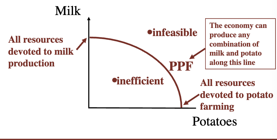
The Production Possibilities Frontier:

• A table or graph indicating all the combinations of goods that an individual or country can produce with a given endowment of inputs and technology
• Example:

• A table or graph indicating all the combinations of goods that an individual or country can produce with a given endowment of inputs and technology
• Assumptions:

- Abstracts the entire economy into two goods

- Snapshot of an economy at one time

• Though the PPF is a snapshot, we can shift it to indicate the effect of changes to an economy’s endowment of inputs and technology
• How would our PPF change with a breakthrough in military technology?

- Improved military tech will allow for more gun production but will have no effect on the amount of domestic goods (“butter”) it can produce. An increase in military tech can allow a society to produce more butter for a given level of guns, since it reduces the amont of resources needed to make that amount of guns

• The PPF indicates all the combinations of goods that an individual or country can produce with a given endowment of inputs and technology (embodies the problem of scarcity)
• Shows the trade-off between producing different goods (the opportunity cost of producing one good in terms of the other
• Opportunity cost of producing each good may differ depending on where an economy sits along the PPF, because different resources are differently suited to producing different goods

- The PPF’s slope will show the marginal rate of transformation between the different goods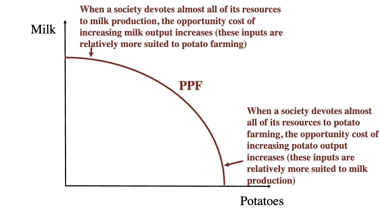

January 17th Notes:

Chapter Two Continued

• Nations’ PPFS will have a bowed shape reflecting the differing opportunity cost at different points along the PPF

The PPF and Opportunity Cost:

• Ex. Crusoe shipwrecked on an island where the only resource is his labor (8 hours). He discovers he can catch 1 fish per hour/harvest 1 coconut every 30 minutes.
• He can devote all 8 hours to coconuts while catching no fish, or spend 8 hours fishing and harvest no coconuts.

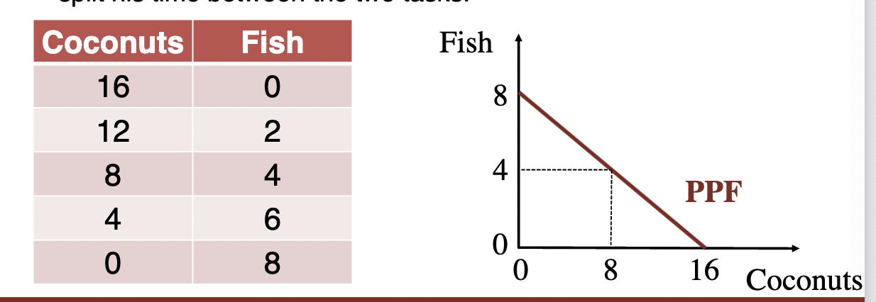
• O.C. of coconut= 8 fish/16 coconuts=½ fish
• O.C. of fish = 16 coconuts/8 fish = 2 coconuts

Absolute Advantage:

• The ability to produce the same good using fewer inputs than another producer.
• Ex. Cruscoue has an absolute advantage in catching fish, and Gilligan in catching coconuts, so they can each specialize.

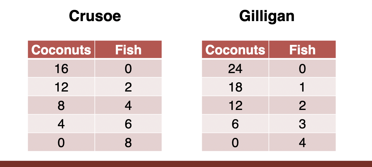
Comparative Advantage:

• The cost of something is what you give up to get it, the opportunity cost for getting it.
• Ex. If Gilligan doesn’t have the absolute advantage for anything say the numbers could conclude:
• Gilligan: O.C. of coconut = 4f/12c = ⅓ fish and O.C. of fish = 12c/4f = 3 coconuts
• Crusoe: O.C. of coconut = ½ fish and O.C. of fish = 2 coconuts
• Even though it takes Gilligan longer to harvest a coconut, he faces a lower O.C. for doing so. This means Gilligan has the comparative advantage in harvesting coconuts because it takes him less time to get a coconut.
• Definition: Producing a good at the lowest opportunity cost compared to other producers
• Rational people will only participate in trades that make them better off. Therefore, trades where the marginal benefit are greater than or equal to the marginal cost.
• Trade can only take place at rates between either party’s opportunity cost of producing both goods for themselves.
• For countries: Comparative advantage means that all countries have a comparative advantage if they produce goods that they can make at a lower opportunity cost.

Absolute and Comparitive Advantage:

• To benefit from trade, a country doesn’t need to have an absolute advantage.
• A country can benefit from trade if it has a comparative advantage and every country will always have some comparative advantage producing something.

Wages:

• Trade raises wages to the highest levels allowed by a country’s productivity (wages will be higher in high-productivity countries than low-productivity countries).

Trade and Globalization:

• Wages rise in high-demand industries and fall in low-demand industries
• Workers will move from low-wage to high-wage industries
• People have differing skills they may have cultivated for whole careers. If no compensation is provided, individuals may thus be hurt as their country embraces free trade.
• At a society-wide level, the gains exceed the losses

Chapter Three-Supply and Demand:

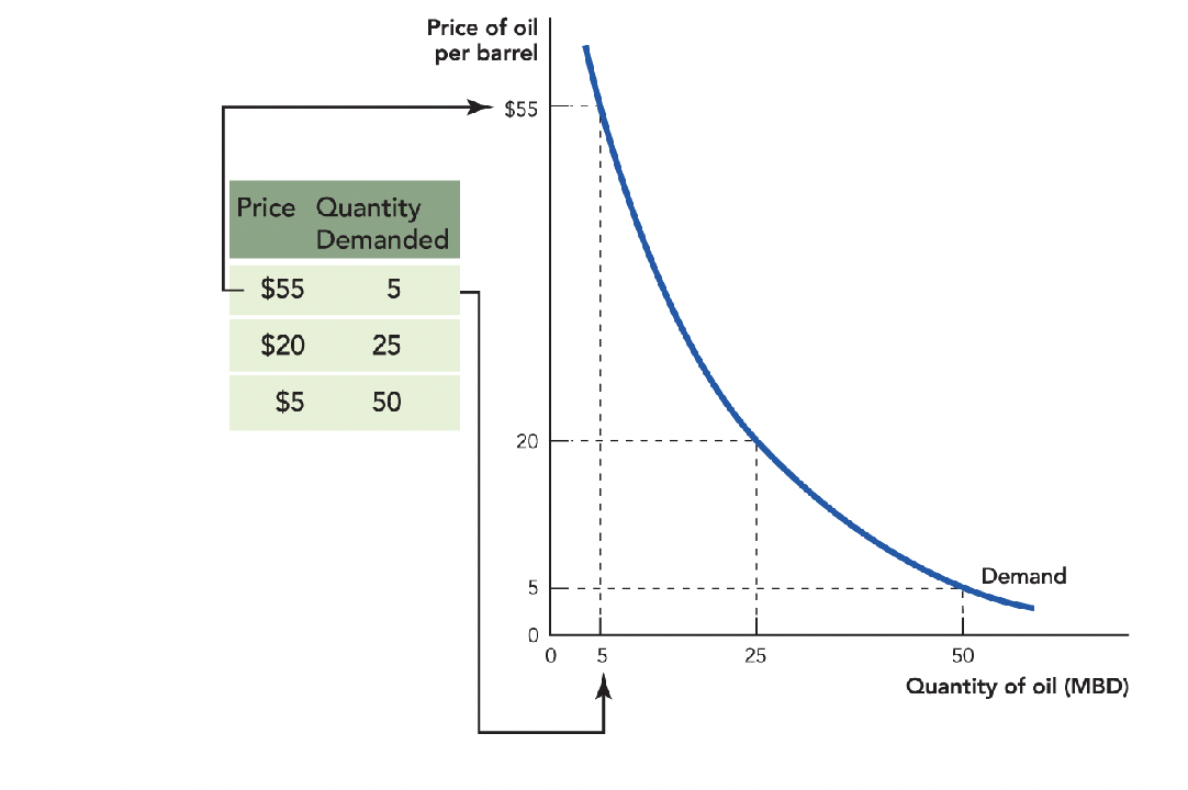
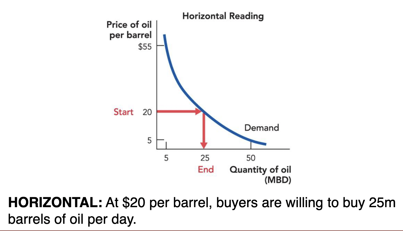
• Demand Curve: A function that shows the quantity demanded at different prices.
• Quantity demanded: The quantity that buyers are willing and able to buy at a particular price.

Demand:

• Data for demand can be used to construct a demand curve

Individual Demand Curve:

• A graph plotting the quantity of an item that someone plans to buy at each price.
• Reflects the question that buyers face everyday: At this price, what quantity should I buy?
• An individual demand curve holds other things constant.
• Ex. Gas costs $3 per gallon, so how much gas should a person buy?

Textbook Notes:

• Economists refer to demand as all possible combinations of prices and quantities in the market.
• What happens to value when a good is transferred from a person who does not value it very much to someone who values it a lot? It increases the value.
• If Kyle voluntarily sells a used guitar to Tona for $800, it must be that:

Tona values the guitar more than Kyle does.

Chapter 1 Review:

Key Terms:

• Incentives: Rewards and penalties that motivate behavior.
• Scarcity: The inevitability of trade-offs is the consequence of a big fact about the world.
• Opportunity Cost: The value of the opportunities lost.
• Great Economic Problem: How we arrange our scarce resources to satisfy as many of our wants as possible.
• Inflation: An increase in the general level of prices.

Other Takeaways:

• It is claimed in the textbook that part of the reason that the Great Depression was so destructive was that economists didn’t understand how to use government policy very well in the 1930s.

Chapter 2 Review:

Takeaway:

• Simple trade makes people better of when preferences differ, but the true power of trade occurs when trade leads to specialization. Specialization creates enormous increases in productivity.
• International trade is trade across political borders. The theory of comparitive advantage explains how a country, just like a person, can increase its standard of living by speciallizing in what it can make at low opportunity cost.

Key Terms:

• Absolute advantage: A country has absolute advantage in production if it can produce the same good using fewer inputs than another country.
• Production Possibilities Frontier: Shows all the combinations of computers and shirts that a country or business can produce given its productivity and supply of inputs.
• Comparitive Advantage: One country/business has the lower opportunity cost in producing a good, so it therefore has a comparative advantage in producing that good.

Chapter 3 Review:

Key Terms:

• Demand Curve: A function that shows the quantity demanded at different prices.
• Quantity Demanded: The quantity that buyers are willing and able to buy at a particular price.
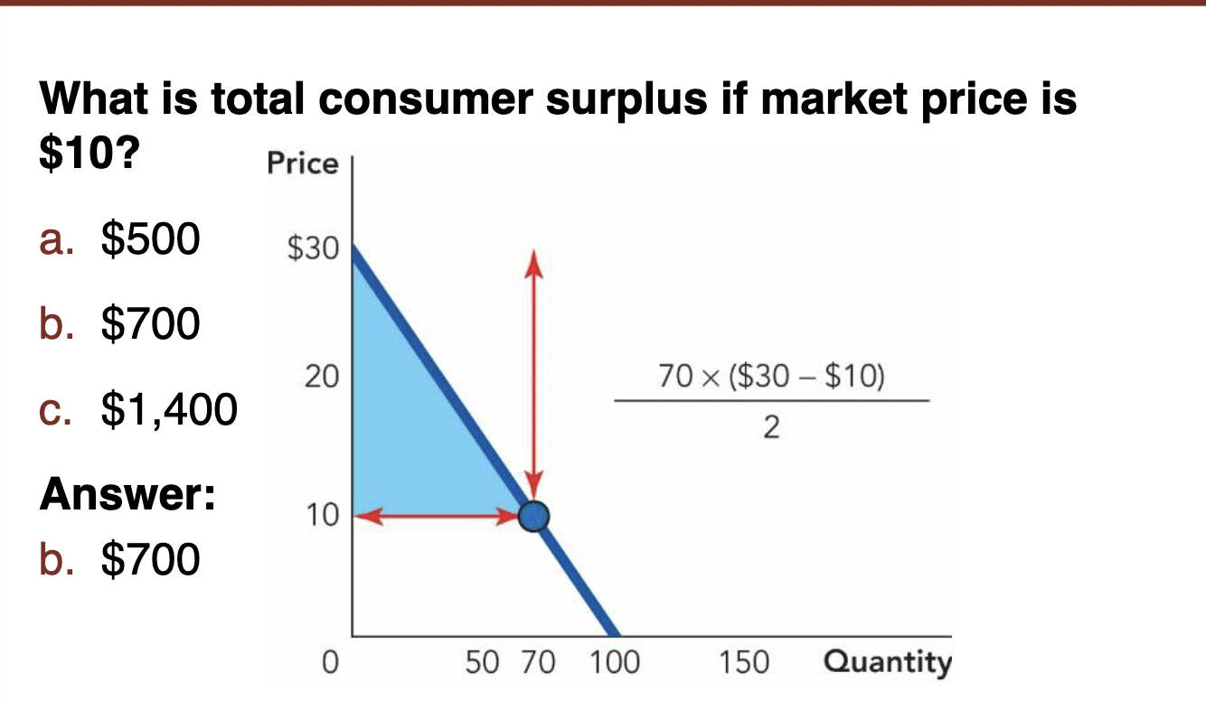
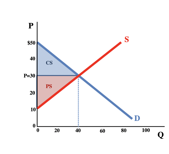
• Consumer Surplus: The consumer’s gain from the exchange.
• Total Consumer Surplus: Found by adding up consumer surplus for each consumer and for each unit. On a graph, it is the shaded area beneath the demand curve and above the price.
• An increase in demand shifts the demand curve outward, up and to the right. On the other hand, a decrease in demand shifts the demand inward, down and to the left.
• Important Demand Shifters:

- Income

- Population

- Price of substitutes

- Price of complements

- Expectations

- Tastes

• Normal Good: When an increase in income increases the demand of a good, we say that good is a normal good.
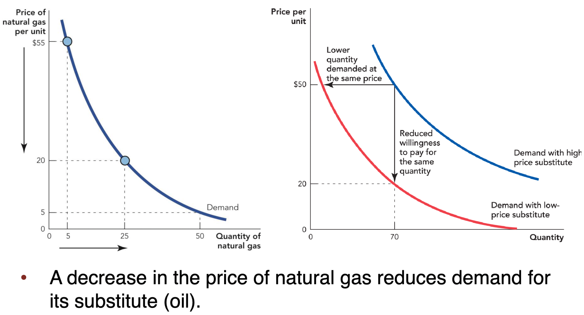
• Substitute: Two goods for which a decrease in the price of one leads to a decrease in demand for the other.
• Complements: Goods that go well together. Two goods for which a decrease in the price of one leads to an increase in demand for the other (ex. Peanut butter and jelly).
• Supply Curve: A function that shows the quantity supplied at different prices. The higher the price, the greater the quantity supplied.
• Quantity Supplied: The quantity that sellers are willing and able to sell at a particular price.
• Total producer surplus: An amount measured by the area above the supply curve and below the price up to the quantity traded.

Takeaways:

• Consumer surplus measures the consumer’s benefit from trade, and producer surplus measures the producer’s benefit from trade.
• Decrease in costs: Shifts the supply curve down and to the right
• Increase in costs: Shifts the supply curve up and to the left
• An increase in supply means that sellers are willing to sell a greater quantity at the same price, or, equivalently, they are willing to sell a given quantity at a lower price.

Quiz:

Go back to 16,18, and 19

January 19th Notes:

Chapter 3-Supply and Demand Continued

• The Marginal Principle:
• Ex. What are Darren’s marginal benefits for each additional gallon of gas?
• Gas is selling for $2.99. As for the marginal principle, Darren would consider each additional gallon of gas separately.
• The cost benefit principle: Darren compared the marginal cost to the marginal benefit for each gallon of gas.
• The opportunity cost principle: When Darren evaluated his marginal benefits, he compared the benefits to the next best alternative.
• The Rational Rule for Buyers: Buy more of an item if its marginal benefit is greater than (or equal to) the price.
• Keep buying until price = marginal benefit

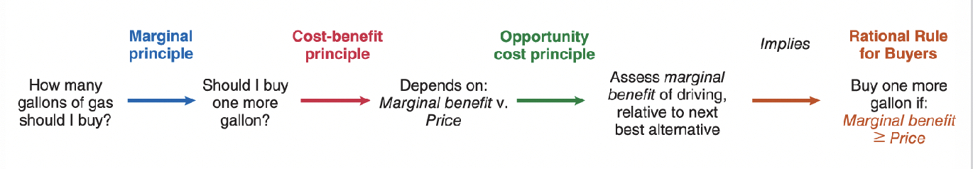
• As buyers experiment, they will typically act as if they follow this analysis, intuitively purchasing goods up to the point where price = marginal benefit.

Holding Other Things Constant:

• When illustrating an individual demand curve, we ask how much we would be willing to purchase at each price, holding other things constant.

- Things other than price can influence demand. Demand for gas, for example, may change if someone buys a more fuel-efficient car.

- Everything is interdependent.

• First, we want to consider what occurs when the price changes.

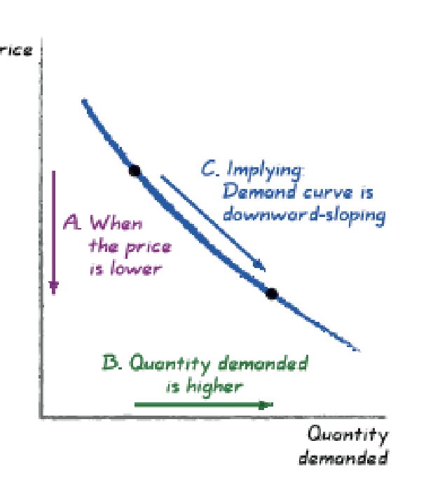
The Law of Demand:

• The quantity demanded is higher when the price is lower - holding other things constant!

Rational Rule

- → price = marginal benefit

- → demand curve = marginal benefit curve

• Diminishing marginal benefit – each additional unit yields a smaller marginal benefit than the previous unit.

Market Demand:

• Market Demand Curve: A graph plotting the total quantity of an item demanded by the entire market, at each price.
• It is the sum of the quantity demanded by each person.
• Individual demand curves are the building blocks of market demand.
• Market demand: The horizontal sum of individual demands

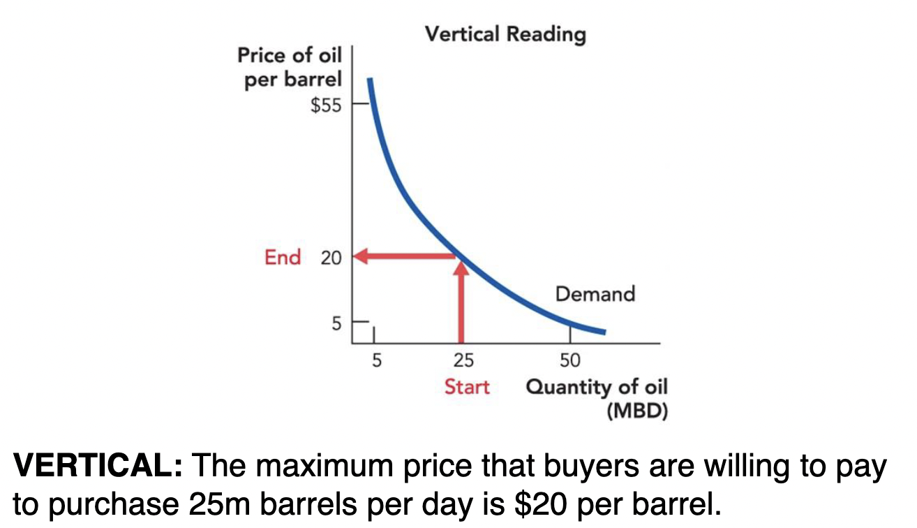
Reading a Demand Curve:

• Horizontally: At a given price, how much are people willing to buy?
• Vertically: What are people willing to pay for a given quantity?

Law of Demand:

• For nearly all goods, the demand curve will always be negatively sloped.
• The lower the price, the greater the quantity demanded
• Demand summarizes how consumers choose to use a good, given:

- Their preferences

- The possibilities for substitution

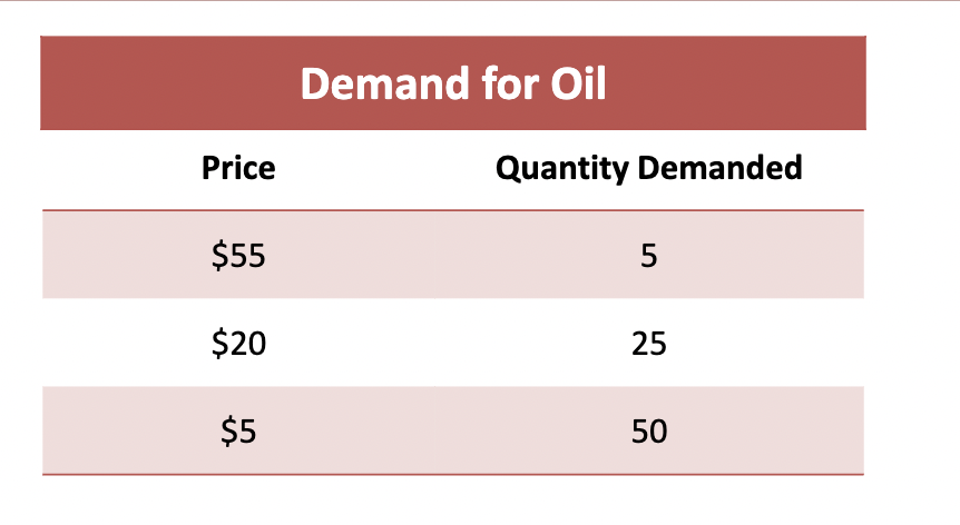
• Consumers will buy more oil at lower prices than at higher prices.
• When the price is high, consumers will use it only in its most valuable uses.
• As the price falls, consumers will also use oil in its less valued uses (ex. Instead of using oil for rubber duckies, can use wood in order to use higher-valued uses of oil for things like airplanes because there is no alternative).

Exceptions:

• Though the law of demand is one of the most fundamental principles in economics, there are a couple of exceptions such as

- Giften goods–cheap necessities, for which an increase in prices might cause consumers to buy more because they can no longer afford luxury substitutes (potatoes in Famine-era Ireland)--and

• Veblen goods– luxury goods whose value lays primarily in conspicuous consumption.
• But these exceptions are such edge-cases we can ignore them for most purposes.

Consumer Surplus:

• Consumer Surplus: The consumer’s gain from exchange; difference between the maximum price a consumer is willing to pay for a certain quantity and the market price.
• Total consumer surplus: The area beneath the demand curve and above the price.
• Example: In the example of Darren deciding how much gas to buy at $3, we would calculate his CS for his first gallon by subtracting this price from his WTP for this gallon ($5-$3=$2). For the second gallon, $4-$3=$1. His total CS would be $2+$1=$3.

January 22nd Notes:

• Change in Demand

- A shift in the demand schedule caused by changes in consumer tastes or conditions

• Movement along the demand curve

- A change in quantity demanded due to the movement from one point on a fixed demand curve to another along the same demand curve caused by change in price.

Factors that Shift Demand:

1. Income

• When people get richer, they buy more
• When an increase in income increases the demand for a good, it is a normal good.
• Most goods are normal goods
• When an increase in income decreases the demand for a good, it is an inferior good.

1. Population

• An increase in population will increase demand generally.
• A shift in subpopulations will change the demand for specific goods and services.

1. Prices of Substitutes

• A substitute is a good that can be consumed instead of another good.
• Your demand for a good will increase if the price of substitute goods rises.
• Your demand for a good will decrease if the price of substitute goods decrease.

1. Prices of Complements

• Complements are things that go well together.
• Your demand for a good will increase if the price of complementary goods decreases.
• Your demand for a good will decrease if the price of the complementary good rises.

1. Expectations

• If you believe prices will rise (or supply will decrease), you will make your purchase today, increasing today’s demand.
• If you believe prices will fall, you will delay your purchase, decreasing today’s demand.

1. Tastes

• Changes in preferences can shift demand curves.

- Companies spend billions of dollars each year attempting to influence our preferences through advertising.

- Social pressure can shift your demand curve

- Preferences are also affected by fads and fashion trends.

Producer Choice and Supply

Supply Curve:

• Supply Curve: A function that shows the quantity supplied at different prices.
• Quantity supplied: The quantity that sellers are willing and able to sell at a particular price.

Reading a Supply Curve:

A supply curve can be read-

• Horizontally: At a given price, how much are suppliers willing to sell?
• Vertically: To produce a given quantity, what price must sellers be paid?

Firm Decisions and the Individual Supply Curve:

Like consumers, firms choose what quantity to produce for markets based on

• The marginal principle
• The cost-benefit principle, and
• The opportunity cost principle

Choosing the best quantity to supply:

• The marginal principle: Decisions about quantities are best made incrementally.
• The cost benefit principle: Decisions depend on the balance of marginal benefits and marginal costs. Produce one more unit if the marginal benefit exceeds the marginal cost.
• The opportunity cost principle: When determining the marginal cost, you should

compare the cost of production to its next best option–not producing.

• Marginal cost does include variable costs …
• Variable costs are those costs that vary with the quantity of output, such as labor and raw materials.
• but does not include fixed costs.
• Fixed costs don’t vary when the quantity of output changes, they are incurred regardless of level of output.

Examples of what to consider when choosing the quantity to supply:

• How many units to supply
• Selling one more unit
• Selling one more unit depends on price versus marginal cost (cost-benefit principle).
• Calculate the marginal cost (opportunity cost principle).
• If the price is greater than the marginal cost, sell one more uniit in order to Maximize Profits!

Rational Rule:

• If maximizing profit, people will always keep selling until the price equals marginal cost.
• The supply curve, therefore, shows the quantity sold at every price, which is also the marginal cost.

Supply Curve Slope:

• The supply curve is upward sloping because of increasing marginal costs.
• As you increase the quantity you produce, the marginal cost of producing an extra unit rises because of the following:

1. Diminishing marginal product leads to rising marginal costs.

• Diminishing marginal product: The marginal product of an input declines as you use more of that input.

2. Rising input costs can also lead to rising marginal costs.

Market Supply Curve:

• A graph plotting the total quantity of an item supplied by the entire market, at each price.
• Market supply is the sum of the quantity supplied by each individual seller.

Law of Supply:

• The tendency for the quantity supplied to be higher when the price is higher (holding other things constant).
• Reflecting the diminishing marginal product, firms will tend to increase the quantity supplied as the price rises.
• As the price of oil rises, it becomes profitable to extract from more costly sources.

Shifts and Movements on Supply Curves:

• When the price changes, you are thinking about a movement along the supply curve.
• When other factors change you need to think about shifts in the supply curve.

Movements along the supply curve:

• A price change causes movement from one point on a fixed supply curve to another point on the same curve.
• Change in the quantity supplied: The change in quantity associated with movement along a supply curve.

Supply Curve Shifts:

• An increase in supply = shift to the right
• At each price, producers are willing to sell more.
• At each quantity, producers are willing to accept a lower price.
• Decrease in supply = shift to the left
• At each price, sellers will offer less
• At each quantity, sellers will demand a higher price

Factors that Shift Supply:

1. Technological Innovations and the Price of Inputs

• Improvements in technology can reduce costs, thus increasing supply. A reduction in input prices reduces costs and thus has a similar effect.

1. Taxes and Subsidies

• A tax on output has the same effect as an increase in costs.
• A subsidy is the reverse of tax

1. Expectations

• Suppliers who expect prices to increase will store goods for future sale and sell less today. The expectation of an increase in price decreases supply and the supply curve shifts to the left.

1. Entry or Exit of Producers

• Shifts the curve down and to the right. This also affects the market supply curve.

1. Changes in Opportunity Costs:

• An increase in opportunity costs shifts the supply curve up and to the left
• If the price of wheat increases, the opportunity cost of growing soybeans increases Some farmers will shift away from producing soybeans and start producing wheat. The supply curve shifts soybeans to the left.

Consumer surplus formula:

½ x (market price-price)xquantity demanded

Producer surplus:

½ x (price given-minimum price) x min quantity demanded

Calculate the area between the price and the supply curve

Chapter Four Notes:

• Surplus: A situation in which the quantity supplied is greater than the quantity demanded.
• Competition will push prices down whenever there is a surplus. As competition pushes prices down, the quantity demanded will increase and the quantity supplied will decrease. Vice versa, competition will push prices up whenever there is a shortage. As prices are pushed up, the quantity supplied increases and the quantity demanded decreases until there is a price where there is no longer an incentive for prices to rise and equilibrium is restored.
• Equilibrium price: The price at which the quantity demanded is equal to the quantity supplied.
• Equilibrium quantity: The quantity at which the quantity demanded is equal to the quantity supplied.
• At equilibrium, neither buyers nor sellers have an incentive to change. At any other point, economic forces push prices and quantities back toward equilibrium.
• Shortage: A situation in which the quantity demanded is greater than the quantity supplied.
• When a free market maximizes the gains from trade, this means:

1. The goods are bought by the buyers with the highest willingness to pay.
2. The goods are sold by the sellers with the lowest costs.
3. There are no unexploited gains from trade and no wasteful trades.

(Together, these three conditions imply that the gains from trade are maximized)

• An increase in supply reduces the equilibrium price and increases the equilibrium quantity.
• An increase in supply = shift of the entire supply curve
• An increase in quantity supplied = movement along a fixed supply curve

Takeaways and Conclusions:

1. Market competition brings about an equilibrium in which quantity supplied = quantity demanded.
2. Only on price/quantity combination is a market equilibrium and this should be identifiable.
3. Should understand and be able to explain the incentives that enforce market equilibrium.
4. The sum of consumer and producer surplus (gains from trade) is maximized at the equilibrium price and quantity, and no other price/quantity combination maximizes consumer plus producer surplus
5. A change in demand is not the same thing as a change in quantity demanded, and the same goes for a supply curve.

January 24th Notes:

Markets:

• Market: A group of buyers and sellers of a particular good or service.
• Competitive Market: A market in which there are many buyers and many sellers so that each has a negligible impact on the market price

—> Price takers buying and selling a homogeneous product

A.K.A. “perfect competition”

Other Market Structures:

• Monopoly: A market with only one seller market

- Seller controls price

• Oligopoly: A market with only a few sellers

- Not always aggressive competition

• Monopolistic Competition: A market with multiple sellers, each selling a slightly different product from its competitors.

What Markets Do:

• Markets organize economic activity by bringing potential buyers into contact with potential sellers.
• They determine:

- what gets produced.

- how much gets produced.

- who produces it.

- who receives it.

- at what price.

• Market outcomes are determined by the forces of supply and demand
• Remember that the demand curve indicated the Qd at each P.
• We can overlay this with the S curve, which shows the Qs at each P.
• The point where the S and D curves intersect shows the P where Qs=Qd

Equilibrium:

• Equilibrium occurs at the price where the quantity demanded equals the quantity supplied

- Equilibrium price: The price at which the market is in equilibrium

- Equilibrium quantity: The quantity demanded and supplied at equilibrium..

• Equilibrium price and quantity are the only factors that are stable in a free market.
• At any other point, economic forces push prices and quantities back at equilibrium.
• (In this class, focus is on equilibrium in perfectly competitive markets.

Adjustment Process: Surpluses

• Consider how markets will reach to a surplus.
• Surplus: A situation in which quantity supplied is greater than quantity demanded.
• Surpluses are seen where the price is greater than the equilibrium price.
• With Qs>Qd, firms will not be able to sell all their inventories.
• Some will lower their prices as they compete for customers.
• This will put a downward pressure on the price, eventually bringing the market to equilibrium.

Adjustment Process-Shortages:

• Shortage: A situation in which quantity demanded is greater than quantity supplied.
• Shortages are seen where the price is lower than the equilibrium price.
• With Qd>Qs, customers will not be able to buy everything they want at the market price.
• Some will offer sellers higher prices as they compete for scarce goods.
• This will put an upward pressure on price.
• Eventually bringing the market to equilibrium.

Equilibrium:

• Occurs when Qd=Qs
• Every buyer who wants the good at the equilibrium price can get it.
• Sellers can sell every unit they want to sell at the equilibrium price.
• Buyers have no incentive to bid up the price.
• Sellers have no incentive to lower prices.

Equilibrium:

• At equilibrium neither buyers nor sellers have an incentive to change.
• At any other point, economic forces push prices and quantities back toward equilibrium
• Equilibrium is the point at which there is no tendency for change.
• Equilibria are also stable in other market structures we discussed, but they will look different.
• There are regular supply- and demand-curve shifts.

- Each S and D curve only shows the Qs and Qd at each price holding all else equal.

- All else does not remain equal–remember all the soruces of S- and D-curve shifts.

• But we will always tend towards the new equilibria.

Equilibrium and Gains from Trade:

• A free market maximizes the gains from trade.

1. Available goods are brought by the buyers with the highest willingness to pay.
2. Goods are sold by the sellers with the lowest costs.
3. Between buyers and sellers, there are no unexploited gains from trade or any wasteful trades.

• These three conditions imply that the gains from trade are maximized.

Welfare Economics:

• Definition: The study of how the allocation of resources affects economic well-being
• The allocation of resources refers to

- how much of each good is produced

- which producers produce it

- which consumers consume it

Consumer Surplus:

• The consumer’s gain from exchange–the difference between the buyer’s willingness to pay for a quantity of a good and the price actually paid for it

- CS=WTP-P

- Total CS is equal to the area under the demand curve but above the price from 0 to Q

Producer Surplus:

• Seller’s gain from exchange–the difference between the price the seller receives for a quantity of a good and the cost of producing it (including opportunity cost)

- PS=P-C

- Total PS is equal to the area under the price but above from 0 to Q

CS, PS, and Total Surplus:

• CS= (value to buyers)-(amount paid by buyers)=buyers’ gains from participating in the market
• PS=(amount received by sellers)-(cost to sellers)=sellers’ gains from participating in the market
• Total Surplus= CS+PS

- = total gains from participating in the market

- = value to buyers - cost to sellers

CS, PS, and Total Surplus

• TS=CS+PS
• Without taxes, notice that:

- TS=CS+PS

- TS=(WTP-P)+(P-Cost)

- TS=WTP-Cost

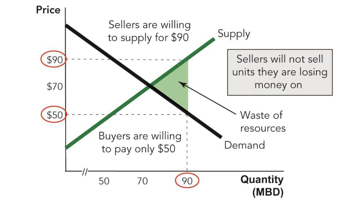
- If Q were below the market equilibrium, both consumers and producers would be worse off for each unit past it

- Beyond Qeq, MB<MC

Total Surplus and Market Efficiency:

• Think about how total surplus would differ if Q were any lower or higher than the equilibrium

Unexploited Gains from Trade:

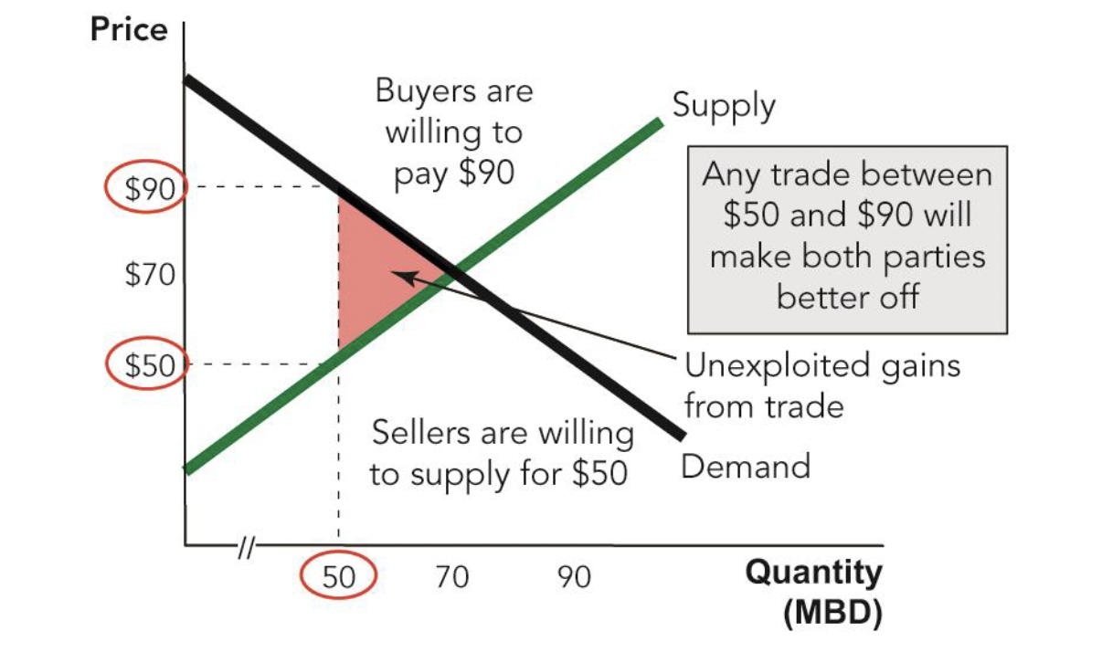
Wasted Resources

• If the quantity traded is less than the equilibrium quantity some gains from trade will be lost.

Another Caveat:

• Free market equilibria may not maximize social welfare in markets with externalities

- Externalities are the uncompensated effects of one person’s actions on the well-being of a bystander

- These effects can be either positive or negative.

• With externalities of consumption, buyers’ demand curves do not fully account for a goods’ marginal benefits.
• With externalities of production, sellers’ supply curves do not fully account for a goods’ marginal costs.
• Thus, their cost-benefit judgements will not result in a socially efficient outcome.
• In markets with externalities, the government can sometimes improve outcomes by implementing policies that help internalize externalities:

- Implementing taxes or subsidies that make people take into account the full cost or benefit of each unit of a good.

- But this requires information that government often lacks, and can be hard to implement.

January 26th Notes:

Negative Externality in Production:

• If production of a good imposes costs on others, the social cost will be above the S curve to account for these external costs.
• The market equilibrium results in too high a Q.

Evidence from the Labratory:

• In fall 1955, Vernon Smith questioned how much the models of perfect competition actually reflect reality.
• In Spring 1956, Smith tested the supply and demand model in a lab

Predicting Market Changes:

1. The consequences of shifts in demand and supply.
2. The ways that changes in prices and quantities reveal whether demand or supply changed.

Set up supply and demand graph

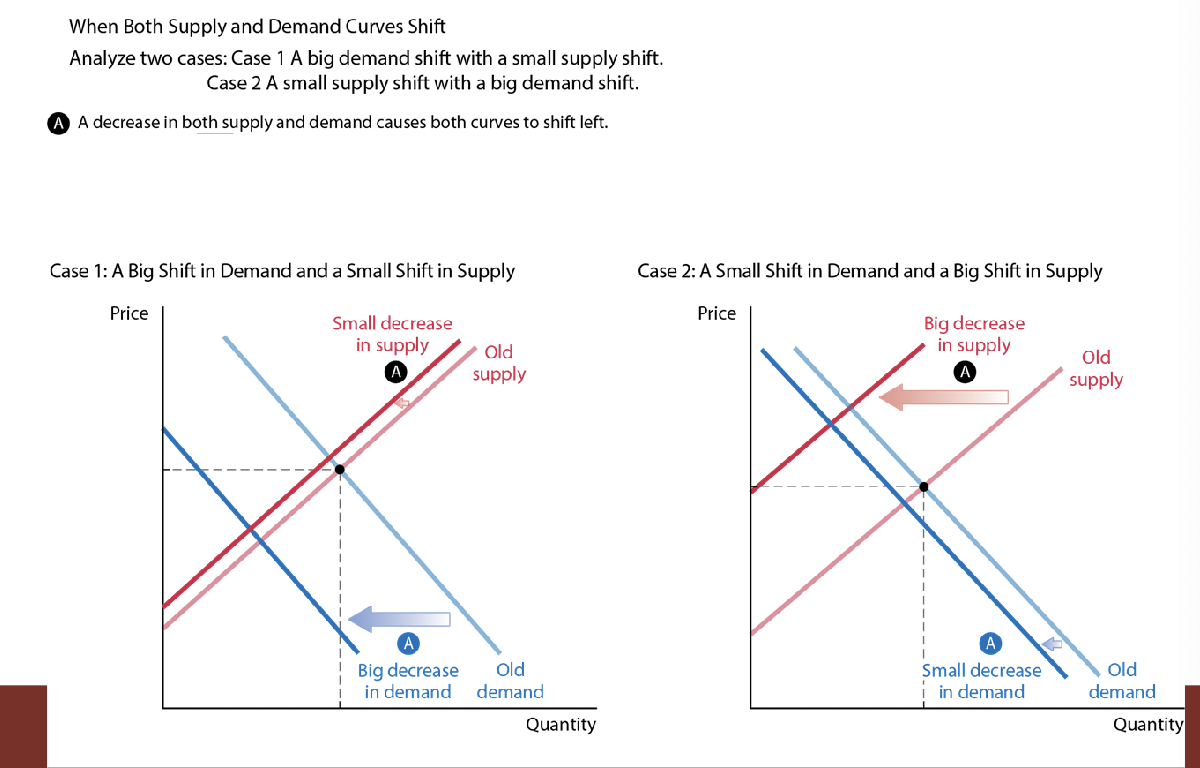
When Both Suply and Demand Shift:

• The conclusion is often unknown/depends on the situation.
• The change in supply might cause the price or quantity to move in one direction.
• The change in demand can cause it to move in the opposite direction.
• Example from the gasoline market:
• The U.S. entered a severe recession, and the price of oil rose sharply.
• A recession reduced the incomes of gas consumers, so demand shifted left.
• Higher oil prices raised costs for gasoline suppliers, so supply shifted left.
• This causes both curves to shift left.
• There was a decrease in quantity in either scenario because supply and demand curves are both shifting, pushing them to lower economies. The demand curve shifts down in price, and supply curve does the opposite.
• When supply and demand both shift, the effect on either price or quantity will be ambiguous

January 29th Notes:

Review:

Chapter 1:

1. Incentives Matter:

• Incentives: Rewards and penalties that motivate behavior
• People respond to all kinds of incentives in predictable ways
• Incentives do not need to be monetary

1. Good Institutions

• When markets work well, individuals pursuing their own interests also promote their self interest, led by an “invisible hand”
• When markets do not work well, government can change incentives with taxes, subsidies, or regulation

Opportunnity Cost Example:

• 70K (from quitting job)+25K (5% interest from 500K)=$95K total opportunity cost
• The day trader’s 100K accounting profit exceeded his 95K opportunity cost. He earned an economic profit of 5K.

Opportunity Costs:

1. Some out of pocket costs are opportunity costs
2. Opportunity costs don’t need to involve out of pocket financial costs
3. Not all out of pocket costs are opportunity costs.
4. Some nonfinancial costs are not opportunity costs.

Sunk Costs:

• Cost that has been incurred and cannot be reversed. Ignore sunk costs.

Thinking on the Margin:

• Choices are made by comparing marginal costs and marginal benefits. Compare the cost of consuming or producing one more unit of a good with the benefit of consuming or producing that one unit.
• Rational people only do something if the marginal benefit is greater than or equal to the cost.
• We ask about individuals’ willingness to pay to obtain the benefits of a particular good or avoid the costs of a particular bad. This willingness to pay is how much you value the good, independent of its market price.

Go over the principles

Ex.

Chapter 2:

Benefits of Trade:

1. Trade makes people better off when preferences differ
2. Trade increases productivity through specialization and the division of knowledge
3. Trade increases productivity through comparative advantage

Specialization:

• Without specialization, each person produces their own food, clothing, and so on.

Division of knowledge:

• With specialization, much more knowledge is used than could exist in a single brain

Production Possibilities Frontier:

• A table or graph indicating all the combinations of goods that an individual/country can produce with a given existing inputs and technology
• Ask how each change would affect the society’s ability to produce each good, if the society specialized entirely in its production.

PPF and Opportunity Cost:

• The O.C. of one thing is the amount of the other that the industry/person does not produce.
• Helpful for understanding what it would look like when one person or industry does not have the absolute advantage in doing anything and to calculate the opportunity costs.

Absolute and Comparitive Advantage

• Countries benefit from trade if they have a comparative advantage rather than an absolute advantage
• Wages rise in high demand countries and fall in low-demand countries.

Market Outcomes:

• Determined by supply and demand
• The point where S and D curves intersect→equilibrium point
• At equilibrium neither buyers nor sellers have an incentive to change
• Economic forces push prices and quantites back toward equilibrium
• Equilibrium is the point where Qs=Qd

Equilibrium and Gains from Trade:

1. Available goods are brought by the buyers with the highest willingness to pay.
2. Goods are sold by sellers with the lowest costs.
3. Between buyers and sellers, there are no unexploited gains from trade or any wasteful trades.

When Supply Increases:

• The S curve shift will cause a movement along the demand curve bringing about a lower price and higher quantity.

When Supply Decreases:

• The S curve shift will cause a movement along the demand curve bringing about a higher P and lower Q

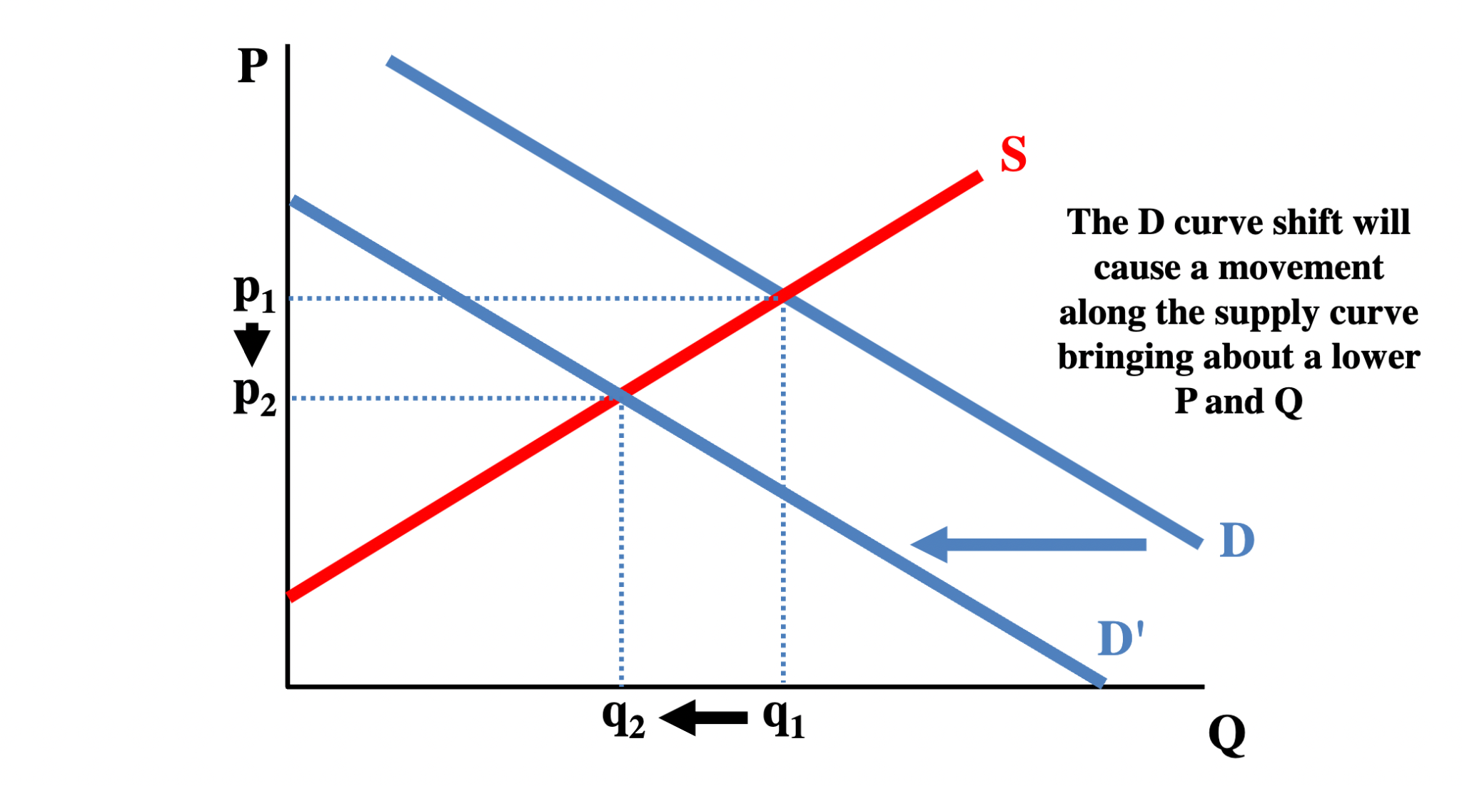
When Demand Increases:

• The D curve will shift and cause a movement along the supply curve bringing about a higher P and Q

When Demand Decreases:

• The D curve shift will cause a movement along the supply curve bringing about a lower P and Q
• 

When Supply and Demand both shift:

• Ex. When supply shifts right and demand shifts down. Small shift in quantity, big shift in price (price shifts down, quantity slightly shifts up)

Chapter 6 Notes:

• Gross domestic product is the market value of all finished goods and services produced within a country in a year. GDP per capita is GDP divided by a country’s population.
• Intermediate goods and services: Some goods and services are sold to firms and then bundled or processed with other goods or services for sale at a later stage.
• The output of an economy includes both goods and services. Services provide a benefit to individuals without the production of tangible output
• Ex: U.S. GDP is about $21.4 trillion, the value of finished services is about $14.5 trillion and the value of finished goods is about $6.8 trillion (68% of GDP is from services so finished goods is 1-0.68=6.8 trillion of GDP).
• Gross national product: Very similar to GDP but GNP measures what is produced by the labor and property supplied by U.S. residents wherever in the world that labor or capital is located, rather than what is produced within the U.S. border.
• Compute percentage change as: (GDP2-GDP1)/GDP1 X 100=GDP growth rate for year 2

Terms with GDP:

• Calculated using prices at the time of sale. It is variables, such as nominal GDP, that have not been adjusted for changes in prices. Therefore, GDP from one year is calculated using that year’s prices. For example, 2018 nominal GDP is found by multiplying 2018 prices and 2018 quantities.
• Real variable: Variables such as real GDP, that have been adjusted for changes in prices by using the same set of prices in all time periods.
• GDP deflator: A price index that can be used to measure inflation. It equals (nominal GDP/Real GDP) x 100.
• Countries with low GDP but a high GDP per capita: UK and France and Country with a high GDP but a low GDP per capita: China

Cyclical and Short-Run Changes in GDP:

• Recessions: Significant, widespread declines in real GDP and employment–are of special concern to policymakers and the public.
• The National Bureau of Economic Reasearch is considered the most authoritative source on identifying U.S. recessions.
• The fluctuations of real GDP around its long-term trend, or “normal” growth rate, business fluctuations or business cycles.
• Business fluctuations: The short-run movements in real GDP around its long-term trend.
• Business Cycles: The short-run movements in real GDP around its long-term trend.

The Many Ways of Splitting GDP:

Two Common ways of splitting GDP-

1. National spending approach to GDP: Y= C+ I + G + (Exports-Imports)
2. Factor income approach to GDP: Y = Employee Compensation + Rent + Interest + Profit

The National Spending Approach:

• Economists have found it useful, especially for the analysis of short-run economic fluctuations, to split GDP into consumption, investment, government purchases, and exports minus imports, which is often shortened to Net Exports.
• Consumption: Private spending on finished goods and services. Most consumption spending is made by households, such as spending on cars and chickens.
• While economists think of education as an investment in “human capital,” the Bureau of Economic Analysis includes education as consumption spending alongside purchases of automobiles, smartphones, and televisions.
• Investment: The purchase of new capital goods; private spending on tools, plant, and equipment used to produce future output. Most investment spending is made by businesses but an important exception is that new home production is counted as investment.
• Government purchases: The third component of GDP. Government purchases is spending by all levels of government on finished goods and services not including transfers. A large part of what government does is transfer money from one citizen to another citizen; about 21% of the spending of the federal government, for example, is for Social Security payments.
• Net exports: Exports minus imports. When we are adding C+I+G, we are adding up all national spending but some of that spending was on imports, goods that were not produced domestically.
• Trade is not ultimately good or bad, but rather that Y=C+I+G+NX is an accounting identity that can’t by itself answer the question of business fluctuation.

The Factor Income Approach:

• GDP can also be written as: Y= Employee Compensation + Rent + Interest + Profit
• When a consumer spends money, the money is received by workers (employee compensation = wages + benefits), landlords (rent), owners of capital (interest), and businesses (profit).
• Not every dollar spent on goods and services is a dollar received in income.
• Employee compensation (wages and other benefits) accounts for about 54% of GDP–more than most people expect and much larger than corporate profits, which are around 10% of GDP.

Problems with GDP as a Measure of Output and Welfare:

• GDP measures the market value of finished goods and services. But we do not know the market value of many goods and services nor do we know the market value of goods and service that are not bought and sold in markets.
• Nations with a great deal of illegal and off-the books activity are not as poor as they appear in the official GDP statistics.
• GDP does not count nonpriced production. Nonpriced production occurs when valuable goods and services are produced but no explicit monetary payment is made. The omission of nonpriced production introduces two biases into GDP statistics: biases over time and biases across nations.
• GDP Does not count bads-Environmental Costs: GDP adds up the market value of finished goods and services, but it does not subtract the value of bads. Pollution, for example, is a bad that is produced every year, but this bad is not counted in the GDP statistics (destruction of water aquifers, the accumulation of CO2 in the atmosphere, or the changing supplies of natural resources are also not counted. For ex, America has cleaner air and cleaner water than it did in 1960, but GDP statistics do not reflect this improvement.
• GDP does not count the health of nations: According to ecnomists Kevin Murphy and Robert Topel, ncreases in life expectancy are worth tens of trillions of dollars, however value of health is not included in GDP.
• GDP does not measure the distribution of income: GDP figures are useful but they will always be imperfect.

Takeaways:

• National spending identity: Y = C+I+G+NX, splits GDP according to different classes of income spending
• The factor income approach: Y = Employee compensation + Interest + Rent + Profit, splits GDP into different classes of income receiving.
• GDP per capita is a rough estimate of the standard of living in a nation. Real GDP is GDP per capita corrected for inflation by calculating GDP using the same set of prices in every year.
• Growth in real GDP per capita tells us roughly how the average person’s standard of living is changing over time.
• GDP and GDP per capita also do not tell us anything about how equally GDP is distributed.
• Economies of Scale: Economies of scale refers to the fact that as production is scaled up, that is, increased quantity, the average cost of producing a good decreases.

Unit 2 Notes:

The law of diminishing returns

thus states that when one input is held constant, increases in the other inputs will begin to yield smaller and smaller increases in output.

February 5th-Chapter 6 Notes:

Introduction:

• Real GDP per capita: A rough measure of a country’s standard of living.

- Switzerland: $91,991.60 (2021)

- Italy: $35,657.50 (2021)

• Switzerland’s residents on average produce 2.6 times as many goods and services as Italy’s.
• Switzerland’s residents can afford 2.6x as much as Italy’s can

Origins of National Income Accounting:

William Petty (1623-1687)

• Hobbes and Empircism
• Down Survey
• Varbun Sapienti
• Political Arithmetick
• The article of the trade of commerce is more of a general piece

Simon Kuznets (1901-1985)

• Wesley Clair Mitchell and Institutionalism: His goal was not to just rely on theory, but rely on as many historical aspects as possible to apply to theory.

- NBER-tool of state trend, allows economists to use statistics reflecting how this will be the basis on how economists collect data. Most use his data or use his theories of collecting data. The origins of modern income accounting.

• “National Income, 1929-1932” (1934)
• National Income and Capital Formation, 1919-1935 (1937)
• National Product Since 1869 (1946)
• Nobel Prize (1971)

Kuznet’s National Income Accounting:

• Decides how much businesses and their owners end up receiving, salaries, withdrawals, how individual entrepreneurs and corporations have business savings or losses, etc.
• Gross Domestic Product: The market value of all finished goods and services produced within a country in a year. Each component is an important part of this definition:

1. Market value

• An economy’s total output includes millions of different goods and services
• Some goods are more valuable than others, so we can’t just add up quantities.
• GDP uses market values to determine how much each good or service is worth and then sums the total.

1. Of all

• As a comprehensive measure, GDP includes everything produced and sold in markets
• The output of an economy includes both goods and services
• Haircuts, medical care, and transportation are some examples of services
• Nonmarket goods and services are not included

1. Finished goods and services

• Only finished goods and services sold to the final consumer are included (ex. A phone)
• Intermediate goods and services used to make another good or service are not included (ex. A silicon chip used to make a phone)
• If intermediate goods were counted, their value would be double-counted

- Counting the silicon chip in itself and as part of the phone would include that chip trice in GDP.

• However, machinery and equipment used to produce other goods are included in GDP
• Any good still on its way to its final transaction to the customer is an intermediate good.

1. Produced

• GDP measures production, so it doesn’t count the resale of existing goods & services (ex. Sale of a used car)
• Second-hand sales change only the ownership of the product
• But the services of the used car dealer getting you in a carry today are new

1. Within a country

• U.S. GDP measures what is collectively produced domestically (within the U.S.)

- This includes products made in the U.S. by foreign-owned businesses.

- U.S. GDP doesn’t include products made in foreign countries by American-owned businesses.

1. In a year

• There needs to be a time frame for GDP
• A year is typically used, although measures are also reported quarterly.

GDP vs. GNP

• GDP: Total output, total spending amd total income in the economy have the same value, which is the economy’s GDP.
• Gross National Product (GNP): The market value of all finished goods and services produced by a country’s permanent residents, wherever they are located, within a year.
• U.S. GDP includes goods and services produced by labor and capitol located in the United States, regardless of the nationality of the worker or property owners.
• GNP is similar to GDP but measures what is produced by the labor and property supplied by U.S. permanent residents
• GNP-GDP = factor payments from abroad - factor payments to abroad

GDP vs. National Health:

• National wealth refers to the value of a nation’s entire stock of assets
• GDP tells us how much the nation produced in a year, not how much it has accumulated in its entire history.
• GDP is calculated by the Bureau of Economic Analysis (BEA), part of the Department of Commerce.

Using GDP:

• And cross-country comparisons

- U.S. $23.3 trillion (2021)

- China $17.7 trillion (2021)

• For measures of prosperity and growth, it is best to use GDP per capita–GDP divided by population

- U.S. $70,243 (2021)

- China $12,556 (2021)

Growth Rates:

• GDP growth rate– the percentage increase in GDP
• Growth rate of GDP for 2018 = [(GDP2018-GDP2017)/GDP2017] x 100
• Using actual numbers (in billions): [($20,580-$19,519)/ $19,519] x 100 = 5.4%
• (GDP 2-GDP1)/GDP1 x 100

GDP per capita growth rate:

• (GDP per capita for previous year-GDP per capita for present year x 100)/GDP per capita growth for previous year
• 0.201

Formulas:

GDP: Y=C+I+G+(Exports-Imports)

Factor Income Approach to GDP: Y= Employee Compensation+Rent+Interest+Profit

Productivity: GDP/workers

Productivity growth rate: (GDP year 2/workers year 2-gdp year 1/workers year 1)/gdpyear 1/workers year 1

Have you calculated productivity by dividing GDP by workers? Then use those numbers to find productivity growth.

February 7th Notes:

Using GDP:

• GDP facilitates cross-country comparisons

- U.S. $23.3 trillion (2021)

- China $17.7 trillion (2021)

• But for measures of prosperity, it is best to use GDP per capita–GDP divided by population

- U.S. $70,243 (2021)

- China $12,556 (2021)

• GDP facilitates itertemporal comparisons
• GDP growth rate-the percentage increase in GDP
• Growth rate of GDP for 2018= GDP2018-GDP2017/GDP2017 x 100
• Using actual numbers for example: $20,580-$19,519/$19,519 x 100 = 5.4%

Real and Nominal GDP:

• Nominal GDP: GDP measured in today’s prices
• Real GDP: GDP measured in constant prices
• The growth rate of quantity is: (QTY-QLY)/QLY
• The growth rate of price is: (PTY-PLY)/PLY

Calculating Nominal GDP and Growth rate:

• NGDP=RGDP+ Price Level
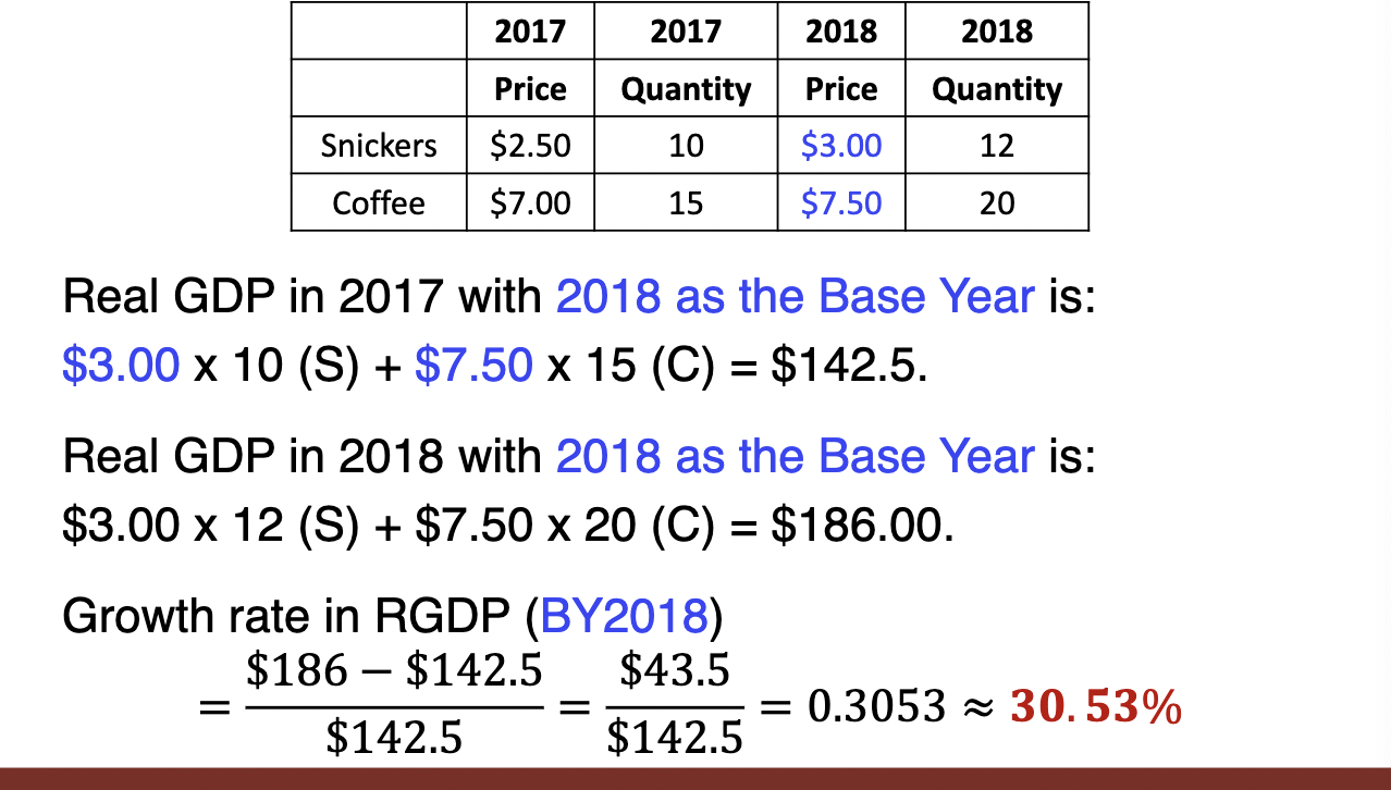
• Base Year: Year at which prices are held fixed (constant) in Real GDP calculation

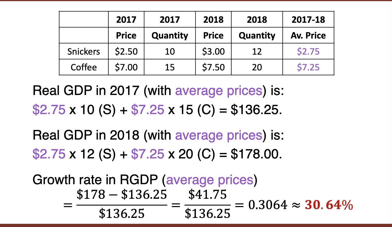
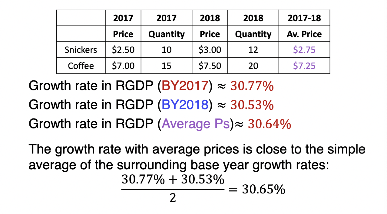
Example of Real GDP Growth Rates with Two Goods:

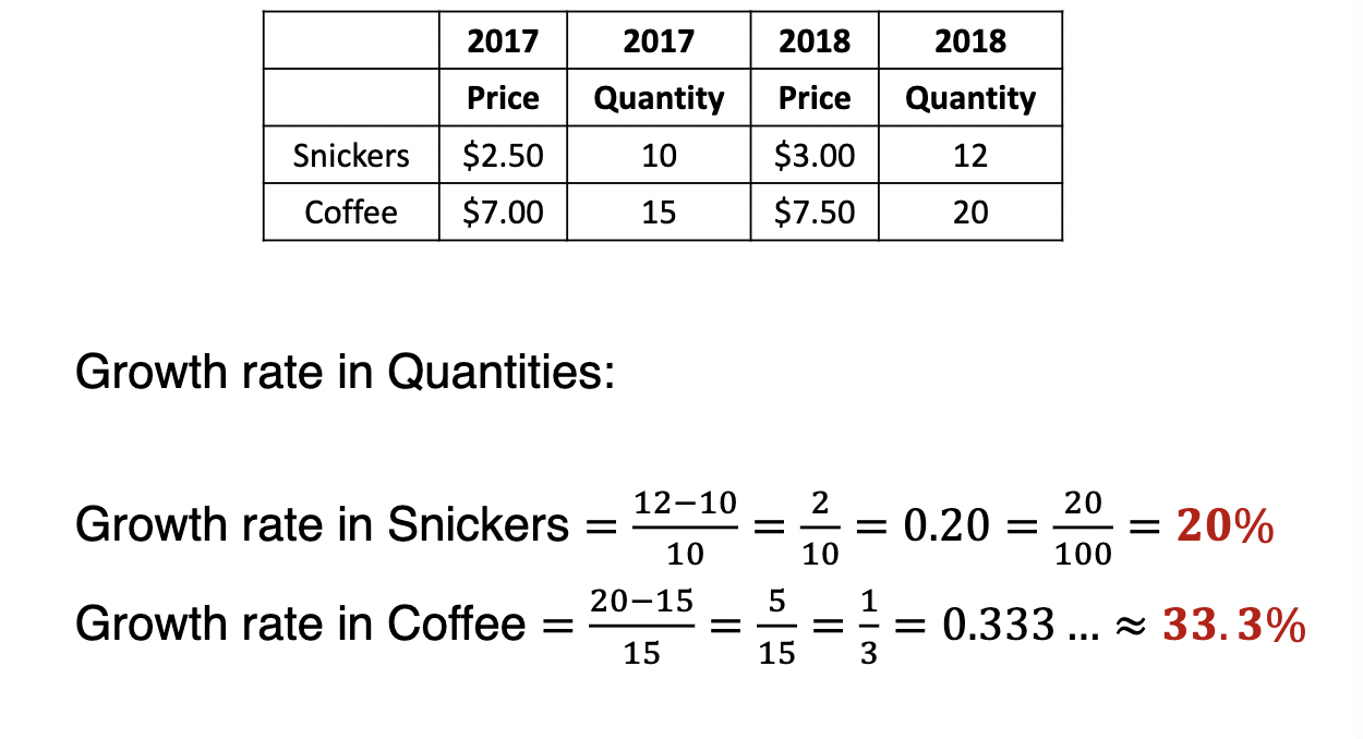
• Nominal GDP in 2017 is: $2.50 x 10(s) + $7.00 x 15(C) = $130.00
• Nominal GDP in 2018 is: $3.00 x 12 (S) + $7.50 x 20 © = $186.00
• Growth rate of NGDP = 186-130/130=43%
• But GR Snickers = 20%, GR Coffee = 33.33%
• Prices increased in addition to quantities increasing! Solution: hold prices constant → real GDP

Real GDP Growth per Capita:

• Real GDP helps control for price changes
• But growth in real GDP does not account for changes in population
• Growth in real GDP will thus overstate economic growth in countries with rapidly growing populations
• Thus growth in real GDP per capita is usually the best reflection of changing standards of living

GDP Deflator:

• Since real GDP controls for price changes, we can use it and the fGDP to measure inflation (the change in overall price levels)
• The GDP deflator is a price index that can be used to measure inflation, calculated by finding the ration of nominal GDP to real GDP (nominal gdp/real gdp x 100)

Nominal GDP versus Real GDP:

• Nominal GDP measures the market value of GDP right now, based on current prices
• Real GDP controls for price changes to measure changes in the quantity of output produced
• Tral GDP per capita is the best measure of economic growth

Short-Run Business Fluctuations:

• GDP is used to compare economic output across countries and over long periods
• GDP is also used to measure business fluctuations or business cycles (short-term movements in real GDP around its long-term trend)
• We call a significant, widespread decline in real GDP and employment a recession
• One popular rule of thumb defines a recession as two consecutive quarters of negative GDP growth.
• But the National Bueau of Economic Reasearch defines a recession as: A significant decline in economic activity spread across the economy, lasting more than a few months, normally visible in real GDP, real income, employment, industrial production, and wholesale-retail sales.

Chapter 7 Notes:

Key Facts About the Wealth of Nations and Economic Growth:

1. GDP per Capita Varies Enormously Among Nations:

• 10% of the world’s population (772 million people) lived in a country with a GDP per capita of less than $2,900 (about the level in Bangladesh). 70% of the world’s population lived in a country with a GDP per capita equal or less than $12,472 (about the level in China), and 73% of the world’s population (5.2 billion people) lived in a country with a GDP per capita less than average. The US is the largest rich country in terms of GDP.

1. Everyone Used to Be Poor:

• In different regions of the world, people were generally poor throughout time. From 1-2000 AD, in the year 1, the GDP per capita was about $700-$1,000. GDP per capita was about the same in year 1 as it would be 1,000 years later, and 1,000 years earlier. For most of human history, there was no long-run growth in real per capita GDP.
• In the nineteenth century some parts of the world began to grow at a rate unprecedented in human history.

A Primer on Growth rates:

• A growth rate is the percentage change in a variable over a given period, such as a year. When we refer to economic growth, we mean the growth rate of real per capita GDP.
• Even slow growth, if sustained over many years, produces large differences in real GDP per capita.
• Ex: If the annual growth rate of real GDP per capita is 2%, how long will it take for real per capita GDP to double from $40,000 to $80,000? Growth builds on top of growth, which is called compounding or exponential growth. To find this, you would use the rule of 70, which is doubling time=70/x years.
• At a growth rate of 2%, GDP per capita will double every 35 years (70/2=35)

1. There are Growth Miracles and Growth Disasters:

• The U.S. is one of the wealthiest countries in they world because it has grown slowly but relatively consistently for more than 200 years. For example, after WW2 Japan was one of the poorest countries in the world. However, from 1950-1970, Japan grew at a rate of 8.5% per year (at that rate GDP per capita doubles in 8 years), and today Japan is one of the richest countries in the world.
• Growth disasters are also possible. For example, Nigeria has barely grown since 1950 and was poorer in 2005 than in 1974 due to high oil prices bumping up its per capita GDP. Argentina was one of the richest countries in the world in 1900 with a GDP 75% that of the US. But, by 1950, Argentina’s per capita GDP had fallen to half of the US, and by 2000 it was less than a third of that of the United States.

Summarizing the Facts:

• Most of the world is poor and more than 1 billion people live on incomes of less than $3 per day. But for most of human history, people were poor and there was no economic growth.
• Economic growth has quickly transformed the world, and has raised the standard of living of most people in developed nations many times above the historical norm. Growth miracles tell us that it doesn’t take 250 years to reach the level of wealth of the U.S.-- South Korea was as poor as Nigeria in 1950, but today has a per capita GDP not far behind Germany or the United Kingdom.
• Growth disasters tell us that economic growth is not automatic either, there are several causes that go into growth miracles and disasters.

Understanding the Wealth of Nations:

The Factors of Production-

• The most immediate cause of the wealth of nations is countries with a high GDP per capita have a lot of physical and human capital per worker and that capital is organized using the best tecnological knowledge to ne highly productive. Physical capital, human capital, and technological knowledge are called factors of production.
• Physical Capital: The stock of tools including machines, structures, and equipments. Some examples are pencils, desks, computers, hammers, shovels, tractors, cell phones, factories, roads, and bridges. Farming is an example of capital: They dig, seed, cut, and harvest using hard labor and simple tools like hoes and ploes. In the US, farmers use a lot more capital–tractors, tricks, combines, and harvesters. The typical worker in the U.S. works with more than $100,000 worth of capital.
• There is also a high tech nature of farming. A tractor’s location is combined with data from other satellites and land-based sensors to adjust the amount of seed, fertilizer, and water to be added to the land. Human capital is tools of the mind; the productive knowledge and skills that workers acquire through education, training, and experience. It is not something we are born with–it’s produced by an investment of time and other resources in education, training, and experience. For example, with farmers, its the human capital that enables them to take advantage of tools like GPS receivers and is why U.S. farmers are more productive (U.S. citizens typically have about 12 years of schooling).
• Technological Knowledge: Knowledge about how the world works that is used to produce goods and services. Includes the genetics, chemistry, and physics that form the basis of the techniques used in modern agriculture. Technological knowledge is increased with research and development, which is potentially boundless. We can learn more and more about how the world works even if human capital remains relatively constant.
• Organization: Human capital, physical capital, and technological knowledge must be organized to produce valuable goods and services.

Incentives and Institutions:

• One example of comparison is North Korea and South Korea. The GDP of South Korea is nearly 20 times higher than North Korea. South Korea has more physical and human capital than North Korea because they have more incentives. In South Korea a worker earns more money if he provides goods and services of value to consumers or if she invents new ideas for more efficient production. In North Korea, workers are rewarded just for being loyal to the ruling Communist Party.
• South Korea uses markets to organize its production much more than North Korea, so they are able to take advantage of all the efficiency properties of markets.
• Incentives matter and good institutions align self-interest with the social interest
• Countries with a high GDP per capita have institutions that make it in people’s self-interest to invest in physical capital, human capital, and technological knowledge and to efficiently organize these resources for production.

Institutions:

• Institutions are the “rules of the game” that structure economic incentives. They include laws and regulations but also customs, practices, organizations, and social mores–institutions are the “rules of the game” that shape human interaction and structure economic incentives within a society.
• Key Institutions include:

- Property rights

- Honest government

- Political stability

- A dependable legal system

- Competitive and open markets

• Institutions create appropriate incentives, incentives that align self-interest with the social interest.

Property Rights:

• Communal property meant that the incentives to invest in the land and to work hard were low.
• There is an incentive not to work and to free ride on the work of others. In the “Great Leap Forward,” the incentive to free ride was made even stronger when communes were increased to 5,000 families. If everyone free rides, the commune will starve. Communal property in agricultural land did not align a farmer’s self-interest with the social interest.
• The Great Leap Foward was essentially a great leap backward because agricultural land was less productive in 1978 than it had been in 1949 when the Communists took over. The farmers agreed to divide the land, which violated governmental policy. The change from collective property rights to something closer to private property rights had an immediate effect: investment, work effort, and productivity increased.
• From 1978-1983 in China, food production increased by nearly 50% and 170 million people were lifted above the World Bank’s lowest poverty line. Property rights in land greatly increased China’s agricultural production. China opened up to foreign investment. Property rights are also important for encouraging technological innovation.

Honest Government:

• Corruption is like a heavy tax that bleeds resources away from productive entrepreneurs. Resources “invested” in bribing politicans and bureaucrats cannot be invested in machinery and equipment, this reducing productivity.
• An honest government is one that spends taxpayer funds on public goods like education, infrastructure, and public health.
• Countries that are more corrupt have much lower per capita GDP.

Political Stability:

• Investors have more to fear than government expropriation.
• Liberia, for example, has had conflict for the past 40 years. Before the election in 2006 of President Ellen Johnson-Sirleaf, it had been 35 years since a Liberian president assumed office by means other than bloodshed.
• In many nations, civil war, military dictatorship, and anarchy have destroyed the institutions necessary for economic growth.

A Dependable Legal System:

• A good legal system facilitates contracts and protects private parties from expropriating one another. In the U.S. for example, it takes 17 procedures and 300 days to collect on a debt. In India, it takes 56 procedures and 1,240 days to do the same thing. This is why it’s relatively difficult for people living in India to borrow money in the first place. Lenders know how hard it is to get their money back.

Competitive and Open Markets:

• The factors of production must not only be produced–they must also be organized.
• The failure to organize capital efficiently has a huge effect on the wealth of nations.
• Half of the differences in per capita income across countries are explained by differences in the amount of physical and human capital.
• Ex: If India used its physical and human capital as efficiently as the U.S. uses its capital, India would be four times richer than it is today. Indian shirts are usually made by habnd in small shops with tailors who design, measure and sow. However, if they were mass manufactured, Indian shirts could be cheaper to make. In the past, in an effort to protect small firms, India prohibited investment in shirt factories from exceeding about $200,000. This meant that Indian shirt manufacturers could not take advantage of economies of scale.
• Economies of Scale: The decrease in the average cost of production that often occurs as the total quantity of production increases.
• In the U.S., it takes about 4 days to start a business, but in India it takes 26, and in Haiti it takes 97 days. Thus, even before a business is begun, an Indian/Haitain entrepreneur must invest extensively in dealing with bureaucracies.

The Ultimate Causes of the Wealth of Nations:

• Institions have a large effect on increasing and organizing the factors of production, and institutions thus have a large effect on economic growth
• Simple natural resources like oil and diamonds are usually good to have but in rich, developed countries, physical and human capital are typically mnuch more important.
• Free trade is not just a matter of policy or choice–it also depends on natural conditions.
• Growth miracle example: The industrial Revolution. This was the first time that human living standards climbed noticeably above the subsistence and stayed there for a long period.
• More wealth in the revolution meant more people could devote their lives to science, invention, and turning new ideas into practical commercial developments. This in turn led to new wealth and then again to more applied science.
• Understanding institutions, where they come from, and how they can be changed is thus a key research question in economics.

Takeaways:

• Today GDP per capita is more than 50 times higher in the riches countries than the poorest
• Poor countries can catch up to rich countries in a surprisingly short period through growth “miracles”.
• What makes a country rich: Countries with a high GDP per capita have lots of physical and human capital per worker, and that capital is organized using the best technological knowledge to be highly productive.
• Countries with a high GDP per capita have institutions that encourage investment in physical capital, human capital, technological innovation, and the efficienty organization of resources.
• Most powerful institutions for increasing economic growth include: property rights, honest government, political stability, a dependable legal system, and competitive and open markets.

February 9th Notes:

Nominal GDP vs. Real GDP:

• Nominal GDP is calculated using prices at the time of the sale

- GDP in 2018 is calculated using 2018 prices.

- GDP in 2017 is calculated using 2017 prices.

• This creates problems when comparing GDP over time.

- We can’t tell if an increase in nominal GDP was due to greater production or increased prices

• Increases in production, not increases in prices, improve the standard of living, so we control for changes in prices with real GDP measures.

Example:

Nominal GDP in 1201 B.C. is:

50 shekels x 22 (I)+16 shekels x 50 (W) = 1,900 shekels

Nominal GDP in 1200 B.C. is:

40 shekels x 20 (I) + 32 shekels x 30 (W) = 2,240 shekels

Growth in NGDP =2240-1900/1900Real GDP:x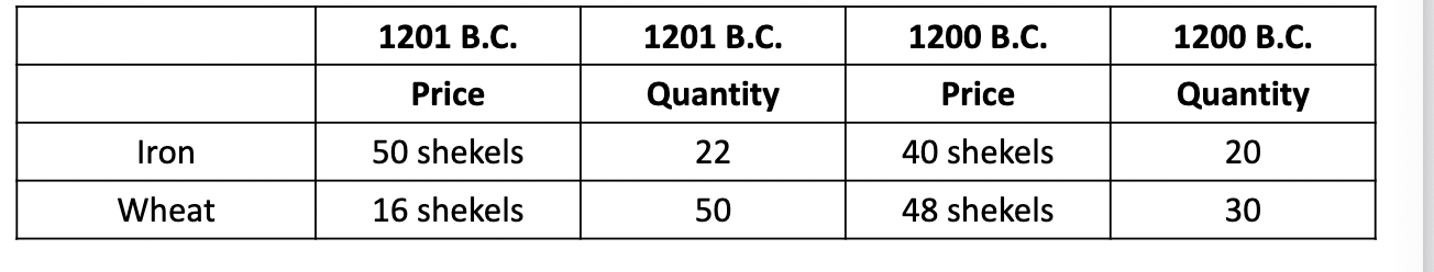

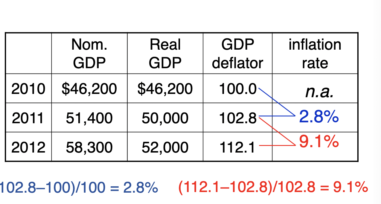
GDP Deflator:

• The GDP deflator (the ration of nominal GDP to real GDP) is a price index that can be used to measure inflation: GDP deflator = nominal gdp/real gdp x 100
• If 2016 nominal GDP + $18.57 trillion, and 2016 real GDP (in 2009 dollars) = $16.66 trillion, GDP deflator = 18.57 trillion/16.66 trillion x 100 = 111.46
• This tells us that 2016 prices were 11.46% higher (111.46-100) than 2009 prices.

The Many Ways of Splitting GDP:

1. National spending approach: Add up the components of spending. Y = C + I + G + (Exports - Imports)
2. Factor income approach: Add up the income generated by producing goods and services. Y = Employee Compensation + Rent + Interest + Profit

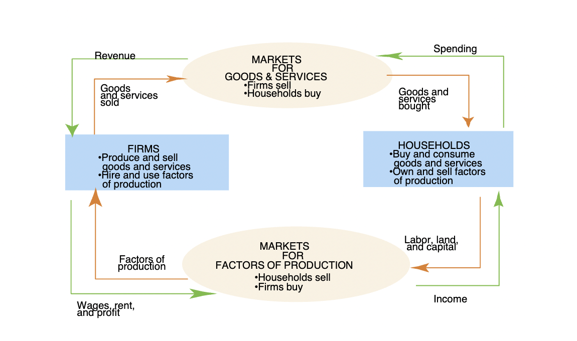
The Circular Flow Model:

• Illustrates the interdependence of the macroeconomy
• Provides a conceptual framework for analyzing macroeconomic interdependence.

An output that’s produced gets sold at some market price → The market value of total output must be equal to total spending.

Every dollar that someone spends is a dollar of income for someone else → Total spending must be equal to total income.

GDP as Total Spending:

• GDP is the sum of consumption, investment, government spending, and net exports.
• Y = C + I + G + NX

Consumption:

• The value of all private spending on finished goods and services
• Includes:

- Durable goods

Last a long time

E.g., cars, home appliances

- Nondurable goods

Last a short time

E.g., food, clothing

- Services

Intangible items purchased by consumers e.g., dry cleaning, air travel

Investment:

• Private spending on capital–private spending on tools, plant, and equipment used to produce future output.
• Includes:

- Business fixed investment

Spending on plant, equipment, and intellectual property

- Residential fixed investment

Spending by customers and landlords on housing units

- Inventory investment

The change in the value of all firm’s inventories

• Consumption includes products made that year/that time

Investment vs. Capital:

• Investment is spending on new capital.
• Example (assuming no depreciation):

- 1/1/2021: Economy has $10 trillion worth of capital

- During 2021: Investment = $2 trillion

- 1/1/2022: Economy will have $12 trillion worth of capital.

Government Spending:

• G includes spending by all levels of government on finished goods and services (including investments)
• G excludes transfer payments like social security checks, unemployment insurance payments, etc.

- These transfer payments do NOT represent spending on goods and services.

Net Exports (NX):

• NX = exports - imports
• Exports: The value of goods and services sold to other countries
• Imports: The value of goods & services purchased from other countries
• Hence, NX equals net spending from abroad on our goods & services

Factor Income Approach:

• GDP is the sum of all incomes in the economy

Y = Employee compensation + Rent + Interest + Profit

• When a consumer spends money, the money is ultimately received by workers, landlords, owners of capital, and businesses
• We can therefore calculate GDP by adding up all the incomes received by workers, landlords, capital owners, and businesses
• When using the factor income approach, adjustments need to be made for things like sales taxes.

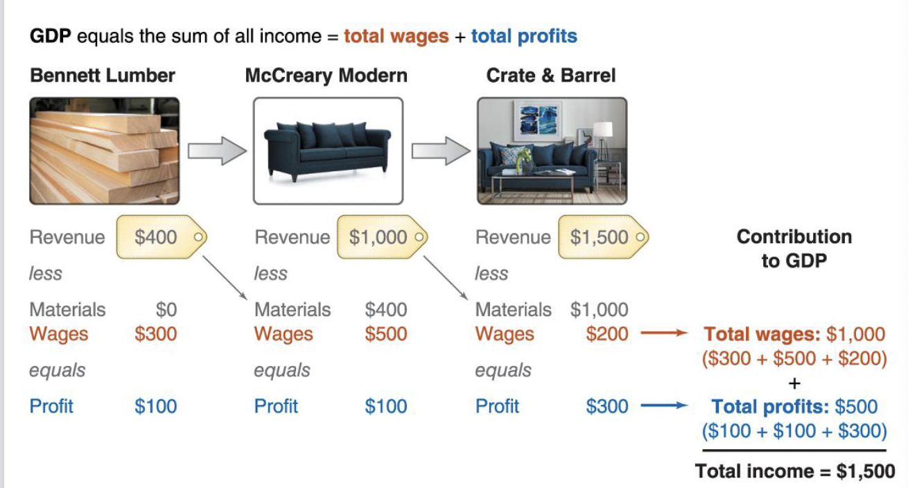
Limitations of GDP:

1. The informal/undergdound economy is missing

• Illegal or underground-market transactions are omitted from GDP
• Underground transactions are especially significant in countries with higher levels of corruption and taxes.
• The informal sector in Latin Ameruca is estimated at 41% of the officially measured GDP
• In the U.S. or Western Europe, the underground economy is likely 10-20% of GDP

1. Nonmarket activities are excluded.

• GDP does not count nonpriced production when valuable goods and services are produced but no monetary payment is made

- Doing housework, reading free blogs, volunteering

• This introduces two biases into GDP statistics: biases over time and biases across nations

- As more women in the U.S. entered the workforce, housework shifted from unpaid to paid.

- Women’s participation in the workforce varies across countries, underestimating the proportion of work included in GDP.

1. Prices are Not Values

• GDP effectively assigns each good and service a value equal to its market price.
• Price may not be a good indicator of value when consumer surplus or a market failure is present.

- Clean water is incredibly valuable, but it is also cheap

1. Nonmarket Prices

• One classic analysis treats the govt’s WWIi spending as solving the Great Depression, but half of spending went to defense–goods and services with no competitive market prices.

1. Reliability of Data

• Macroeconomic measures are only as good as the data used to construct them.
• Measures can also be unreliable in countries with limited transparency.

1. Measures Goods but not Bads:

• GDP adds up the value of finished goods and services but does not subtract the value of “bads”:

- Pollution

- Changing supplies of natural resources

- Loss of animal or plant species

- Crime

• “Green accounting” attempts to cover the environment more explicitly.
• Environmental amenities are difficult to value.

1. Omitted Measures of Well-Being:

• GDP does not count the health of nations
• GDP does not count the value of leisure

- GDP includes the benefit of work, which is more income

- GDP does not include the cost of work, which is less leisure

1. GDP as a Measure of Living Standards

• GDP leaves out a lot, but the GDP per capita is still the best measure we have of economic prosperity
• Economicaly prosperous societies enjoy more than just material goods:

- Higher infant survival rates, life expectancy, education, etc.

- They also face fewer civil wars, riots, and social conflicts.

• GDP indicates the resources available to pursue things people value.

Chapter 7 Notes:

• Economically prosperous societies enjoy more than just material goods.
• Economic growth is the engine of prosperity:

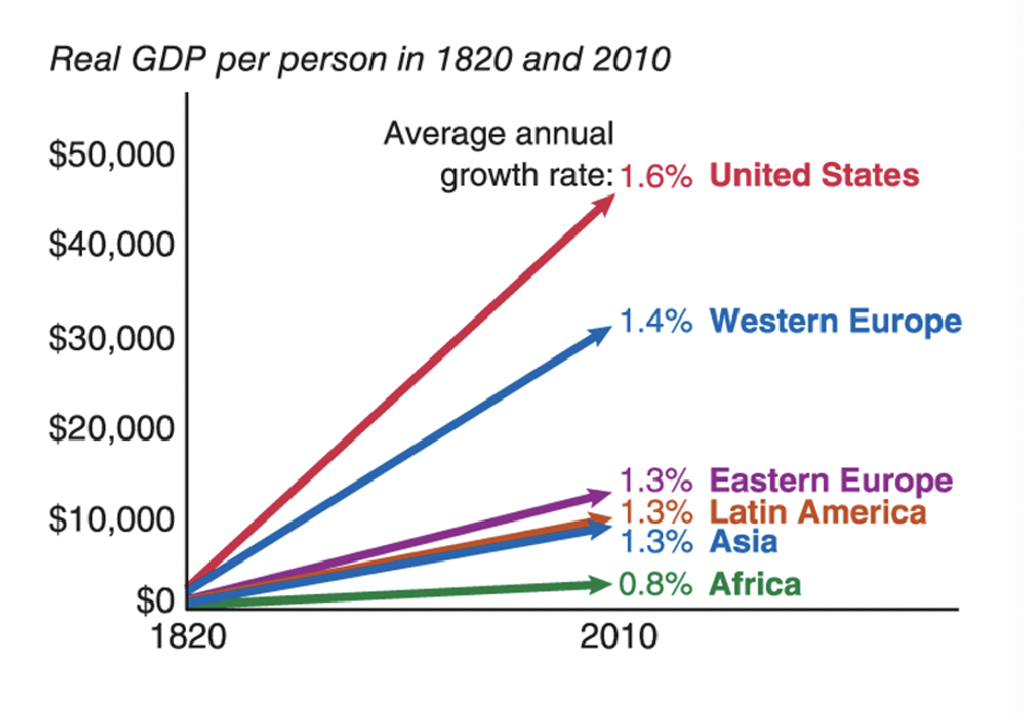
Key Facts:

• Key facts about the wealth of nations and economic growth:

1. GDP per capita varies enormously among nations
2. Everyone used to be poor
3. There are growth miracles and growth disasters.

GDP Per Capita Varies:

• Around 75% of the world’s population lives in a country with an annual GDP per capita less than the world average
• Poverty is normal: It is the default option.
• It is wealth that is unusual

Everyone Used to Be Poor:

• GDP per capita from the Classical Age through 1000 A.D. is estimated at around $700-$1,000 per year in 2015 dollars.
• This was approximately the same in all major regions of the world.
• For most of human history, there was no long-run growth in real per capita GDP.

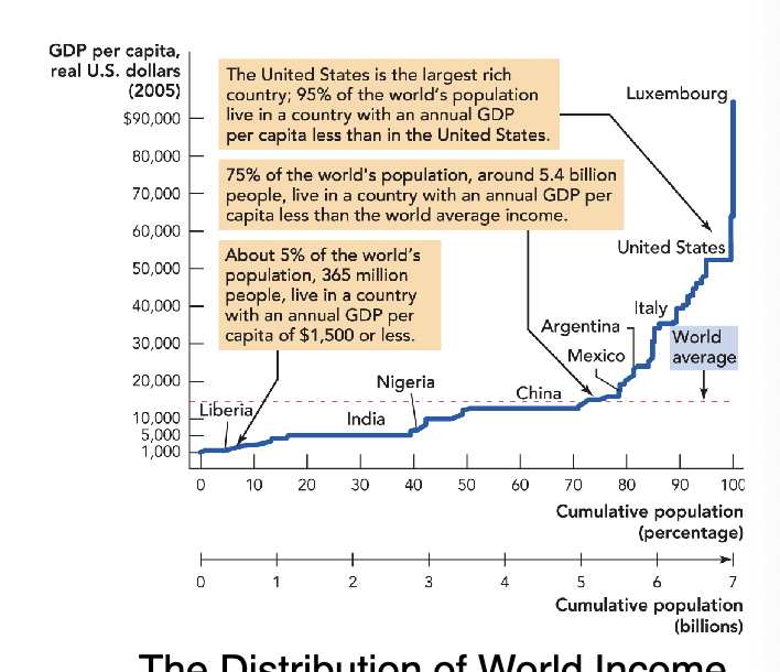
The Start of Modern Growth:

• England went from about $700 in income per capita, to $1,000, to a higher increase by 1750. However, they had a small growth rate of 0.03%.
• But, they continued to become richer than they started and kicked off modern economic growth

Measuring Growth:

• Economic growth is measured as the growth rate of real GDP per capita: gt=yt-yt-1/yt-1 x 100
• Where:

Gt = growth rate of real GDP per capita

Yt = real GDP per capita in time period t

• Example: 2021 real gdp per capita is 13,770 pounds and 2022 real GDP per capita is 14,600 pounds, therefore:

gt=(14,600-13,770)/(13770) x 100 = 6.0%

• Growth builds on top of groth through “compounding” or “exponential growth”.
• Thus, even slow growth produces big differences in wealth if sustained over time.
• The rule of 70 approximates the length of time necessary for a growing variable to double:

Doubling time = 70/growth rate in %

• Example: If real GDP per capita is growing at an annual rate of 2%, it will double in: 70/2 = 35 years.
• Thus, we can see that even if our GDP per capita were just a little bit smaller growth will be much slower:

70/1.4 = 50 years

Why Does Growth Matter?

• Before modern civilization, there was little to no economic growth with every generation living the same as its ancestors.
• Early-modern agricultural improvements allowed more non-farm activity, allowing for an intensified division of labor, setting the stage for the Industrial Revolution– which accelerated growth rates
• Small differences in economic growth amplify over time, resulting in “rich” countries. (Rule of 70)
• Health (mortality & longevity) improved dramatically.

Developed Countries:

• The United States is one of the world’s wealthiest countries because it grew slowly but consistently for more than 200 years.

Undeveloped/Developing Countries:

• Poverty is normal.
• Without growth, any country will not increase its prosperity.
• Without very favorable conditions, even poor countries’ growth will often be slow or unstable.

Japan:

• From 1950 to 1970, Japan grew 8.5% per year.

- Now it’s one of the richest countries in the world

• Continued growth is NOT guaranteed

Other Growth Miracles:

• In 1950, South Korea had GDP per capita about the same as that of Nigeria.

- From 1970 to 1990, it grew at a rate of 7.2% per year.

- Today, South Korea is on par with many European economies

Argentina:

• In 1900, Argentina was one of the richest countries in the world, with GDP per capita almost as large as that of the United States.
• After the Saenz Pena Laws introducing universal male suffrage in 1912, Argentina faced unstable political institutions.
• By 1950, Argentina’s per capita GDP had fallen to half that of the U.S.
• By 2000, Argentina’s per capita GDP was less than one-third that of the U.S.
• Arguably the only good example of a rich country becoming poor.

Other Growth Disasters:

• Nigeria has barely grown since 1950.

- It was poorer in 2005 than in 1974, when high oil prices briefly bumped up its per capita GDP.

Economic Growth:

Bad News:

• Most of the world is poor.
• More than 1 billion people live on incomes of less than $3 per day.
• These people have greatly reduced prospects for health, happiness, and peace.

Good News:

• Despite being a quite recent phenomenon, economic growth has transformed the world.
• It has raised the standard of living of most people in developed nations many times above the historical norm.
• Understanding the wealth of nations is critical if we are to improve the human condition.

Understanding the Wealth of Nations:

• The causes of growth in GDP per capita include factors of production, incentives, and institutions.

Factors of Production:

• Firms combine various inputs–or factors of production–when making their outputs.
• At the macroeconomic level, we will group these factors of production as labor, human capital, physical capital, and technological knowledge.

Physical Capital:

• The stock of tools used in the production of goods and services, which includes machines, structures, and equipment.
• This capital stock determined by past investment.
• You are more productive when you have the right equipment.

- Physical capital is a complement to labor in production.

Labor and Human Capital:

Labor is the amount of time that workers spend on the job.

• The more labor that workers do, the more output gets produced.

- Thus, a population increase will boost GDP but not GDP per capita.

Human capital is the productive knowledge and skills that workers acquire through education, training, and experience.

• The more human capital a worker has, the more output he can produce per hour.

- Thus, increased human capital will increase labor productivity.

Output reflects the quantity of hours worked and the productivity of people at work.

• Labor productivity is the quantity of goods and services that each person producers per hour of work.
• Your labor productivity depends in part on your human capital as well as the other factors of production at your disposal.

- Labor, human capital, and physical capital are complements in production.

Demographics and Growth:

• The dependency ratio is the number of people too young or too old to work per 100 people of working age.
• The dependency ratio rose sharply due to the post-WW11 baby boom
• Low fertility rates and growing life expectancies mean it will rise again.
• Women entered the labor force in large numbers duringh WWII.
• Women were responsible for a large share of the growth in measured per capita GDP

- GDP does not count non-market work

February 14th Notes:

Growth is not always guaranteed:

Argentina:

• In 1900, Argentina was one of the richest countries in the world, with GDP per capita almost as large as the United States
• After the Sáenz Peña Laws introducing universal male suffrage in 1912, Argentina faced unstable political institutions.

Understanding the Wealth of Nations:

• The causes of growth in GDP per capita include factors of production, incentives, and institutions.

Technological Knowledge:

Technological knowledge is the knowledge about how the world works that is used to produce goods and services.

• New methods for existing resources
• Makes it possible to produce more from given resources.
• Better technological knowledge has allowed U.S. farms to increase their output two and a half times since 1950, and while using less land.
• Unlike the physical capital of a new combine or a specific farmer’s human capital in knowing how to use it, the knowledge about how to build this combine can be shared by everyone
• Improved technological knowledge increases productivity (the amount of output we can get from given inputs) and is thus potentially boundless.

A country will produce more output if:

1. It employs more workers
2. Its workers become more highly skilled.
3. It accumulates more physical capital.
4. It develops technological knowledge allowing it to use the other factors of production more efficiently.

Institutions:

Institutions are the “rules of the game” that structure economic incentives.

• A country’s institutions not only include its legal and regulatory regime but also its customs, practices, organizations, and social mores.

Incentives and Institutions:

• Institutions that promote growth create incentives that align self-interest with the social interest.
• Wealthy countries have institutions that make it in people’s self-interest to invest in physical capital, human capital, and technological knowledge.

Institutions of economic growth include:

• Property rights
• Honest government
• Political stability
• A dependable legal system
• Competitive and open markets

Property Rights:

• Property rights grant control over a tangible or intangible resource.
• Property rights are important institutions for encouraging investment in physical and human capital.
• Under communal property, effort is divorced from payment, so there is incentive to free ride.

- A free rider is someone who consumes a resource without working or contributing to the resource’s upkeep.

Property Rights:

• War Communism and the New Economic Policy: Farmers would only make enough for themselves to survive
• Spain’s Mesta:
• Savers won’t save and investors won’t invest if they don’t expect that they will receive a return for their savings and investment.
• Property rights are also important for encouraging technological innovation.
• Companies will not undertake research and development unless they expect to profit from it.

Honest Government:

• Corruption is like a tax that bleeds resources away from productive entrepreneurs.
• Resources “invested” in bribing cannot be invested in machinery and equipment.
• Corruption makes it more profitable to be a corrupt politician or bureaucrat.
• Few people want to be entrepreneurs because they know that their wealth will be stolen.

Political Stability:

• Like corruption, political instability discourages investment and innovation.
• In many nations, civil war, military dictatorships, and anarchy have destroyed the institutions necessary for economic growth
• After the Sáenz Peña Laws introducing universal male suffrage in 1912, Argentina went through populist governments, a military coup in 1930, Juan Peron’s election as a populist in 1946, 1955’s Rvolucion Libertadora, etc.

Dependable Legal System:

• A good legal system facilitates contracts and protects private parties from expropriating one another.
• Poorly protected property rights can stem from e
• ither too much or too little government.
• Some legal systems are of such low quality that no one knows for certain who owns what.
• It is difficult to borrow money if lenders aren’t sure they will get their money back.

Competitive and Open Markets:

• About half of the differences in per capita income across countries are explained by differences in the amount of physical and human capital.
• The other half of the differences are explained by a failure to use capital efficiently,
• Competitive and open markets are one of the best ways to encourage the efficient organization of resources.
• Some reasons for inefficient organization include:

- Inefficient and unnecessary regulations

- Red tape, or the time and cost to do tasks such as starting a business or enforcing a contract in a court of law

- Barriers to free trade

Government Policy to Encourage Innovation and Economic Growth:

As we’ve seen technological knowledge is a potentially boundless source of economic growth.

Like other factors of production, investment in new technological knowledge is subject to the incentives created by our institutions.

Government strategies to encourage innovation include the following:

1. Create incentives through intellectual property laws.
2. Subsidize research and development

February 16th Notes:

Ultimate Causes of Wealth:

• Natural resources may help explain why a country is able to accumulate physical and human capital
• Transport is cheaper over water than over land, so countries with access to water are more open to trade
• Landlocked countries have lower per capita GDP than countries with access to a coast.
• But plenty of resource-rich countries are poor.
• History, ideas, geography, culture, and luck are also important to economic growth.

Chapter 8:

Introduction:

In 2010:

• China’s GDP per capita grew nearly 10%.
• U.S. GDP per capita grew by 2.2%

China is growing much faster than the United States because:

• The Chinese economy is catching up.
• The U.S. economy is on the cutting edge.

Cutting-Edge Growth vs. Catch-Up Growth:

Catching-up growth:

Growth due to capital accumulation.

• With very low capital per worker, the marginal product of capital will be very high–allowing rapid growth through capital accumulation.

Cutting-edge growth:

Growth due to new ideas.

• With higher levels of capital per worker, the marginal product of capital will be lower–meaning that growth will depend on new ideas about how to use factors of production more efficiently.
• Japan 1950-1970: 8.5% annually for 20 years
• Japan since the 1990s: ~1% annually

Solow Model:

• Grouping factors of production as labor, human capital, physical capital, and technological knowledge
• We can also represent how these factors of production contribute to total output mathematically.
• A production function expresses a relationship between output and the factors of production:

Y = f(A,K,eL)

Where the total output of an economy (Y) depends on:

• Physical capital (K)
• Human capital, or education x labor (eL)
• Technological knowledge or ideas (A)
• If we assume that A, e, and L are constant, then we can simplify our expression for output as: Y = F(K)
• More capital (K) should produce more output (Y), but at a diminishing rate.
• Because L is constant

- An increase in K always implies an increase in the amount of capital per worker, K/L.

- An increase in Y is also always an increase in output per worker, Y/L (AKA Productivity)

The Law of Diminishing Returns:

• Capital, labor, and human capital are complements in production.
• While holding all other inputs constant, the marginal return on nay input will thus decrease as we intensify its usage.
• Thus, the law of diminishing returns states that when one input is held constant, increases in the other inputs will, at some point, begin to yield smaller and smaller increases in output.

Capital, Production, and Diminishing Returns:

• If we hold labor (L), human capital (e), and technological knowledge constant (A), the law of diminishing returns applies to capital (K) in our production function: Y = f(A,K,eL)
• Thus, more capital (K) should produce more output (Y) but at a diminishing rate even in our simplified production function: Y = F(K)

Marginal Product of Capital:

• Economists think in marginal terms.
• Consider the costs and benefits of consuming or producing one more unit of a good.
• The marginal product of capital (MPk) is the increase in output caused by adding one more unit of capital.
• The MPk at K=0 is the increase in output from adding the first one unit of K beyond 0: square root of 1-square root of 0= 1-0 = 1
• Likewise the MPk at K = 15 is the increase in output from adding one unit of K beyond 15: square root of 16 - square root of 15 = 4-3.87 = .13
• This graph shows the production function Y = F(K): In this case, output is the square root of the capital input = square root of K. If K = 4, then Y = square root of 4 = 2. If K increases to 16, then Y = square root of 16= 4.

Applying the Solow Model to China:

• Chinese growth has been rapid for the following reasons:
• China began with very little capital, so its marginal product of capital was high.
• With new reforms, the investment rate increased dramatically.
• China has benefited by opening up to trade and investment with the developing world.
• Chna has improved its productivity in agriculture.
• China’s growth rate will eventually fall for the following reasons:
• The marginal product of capital will fall.
• It has a poor banking system
• It lacks experience with the rule of law
• It has a poorly educated population

Capital and Investment:

• Capital is past output that was saved and invested rather than consumed
• We model investment in capital as a fixed fraction of output, so for example 3/10=0.3

Capital and Depreciation:

• Capital also depreciates (wears out). For example, if there are 100 units of capital, 2 units might depreciate, labing 98 for the next period.
• The greater the capital stock, the greater the depreciation–placing a constraint on economic growth.

Chapter 8 Notes:

Two Types of Growth:

• Catching Up: Growth due to capital accumulation and adopting already existing ideas.
• Cutting-edge:
• Growth due to new ideas. Countries that are catching up have many enormous advantages. In order to become rich, a poor country doesn’t have to invent new ideas, technologies, or methods of management.
• The U.S. is the world’s leading economy–it’s on the cutting edge
• Growth on the curing edge is primarily about developing new ideas. When thinking about growth in the United States, we think about things like iPhones, the Internet, and genetic engineering.

The Solow Model and Catching-Up Growth:

• The solow model begins with a production function. This expresses a relationship between output and the factors of production, namely the exact way in which more inputs will produce more outputs.
• Assume there is only one output Y, which we can think of as GDP, and the three factors of production are: physical capital, written K; human capital (eL), and education (e), times labor (L); and ideas that increase the productivity of capital and labor (technical knowledge), which we write as A. Y=F(A,K,eL)
• Example: For a typical production process, like an automobile factory, output depends on capital (the machines K), labor (the workers L adjusted for their level of skill, so eL), and the ideas upon which the whole factory is based (a), namely the invention of the auto and all the machines that help make it.
• If L (the number of workers) is constant, for example, an increase in K (capital) always pimples an increase in the amount of capital per worker, K/L and an increase in Y (output) is also always an increase in output per worker, Y/L.

Capital, Production, and Diminishing Returns:

• More capital, K, should produce more output, Y, but at a diminishing rate. For example, on a farm, the first tractor is very productive. The second tractor is still useful, but not as much as the first tractor. The third tractor is driven only when one of the other tractors breaks down (the amount of labor is constant.
• When there are increased in capital, produce less output, Y, the more capital you already have–so the production function in which output increases with more output but at a decreasing rate.

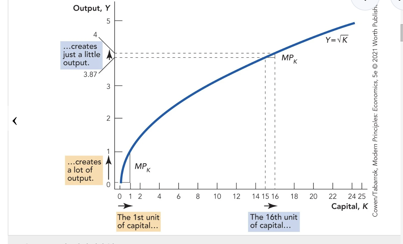
• The first unit of capital increases output by one unit, but as more and more capital is added, output increases by less and less– this is the “iron logic” of diminishing returns and it plays a key role in the Solow model.
• Marginal product of capital: The increase in output caused by the addition of one more unit of capital; the marginal product of capital diminishes as more and more capital is added. Y = F(K) = square root of K, which means that output is the square root of the capital input. Ex., If K = 4, then Y = square root of 4 = 2. If K increases to 16, then Y = square root of 16 = 4 and so forth.
• In a country without a lot of capital but good institutions, the marginal product of capital will be very high. Even small investments pay big rewards and economic growth will be rapid.

China:

• For most of the twentieth century, China labored under very poor economic institutions.
• Since the death of Chairman Mao in 1976 and the subsequent move away from Communish and toward markets, China has been growing very rapidly. Chinese growth has been rapid because China began with very little capital, so the marginal product of capital was very high, and with the new reforms the investment rate increased dramatically.
• China also grew rapidly because improved productivity in agriculture brought about primarily by better institutions–prompted several hundred million Chinese rural peasants, who were no longer needed to work the land, to migrate to Chinese cities.
• China is catching up to the states, but growth in China will slow. China’s growth rate will fall because the marginal product of capital will fall. The country also has several issues regarding a poor banking system and a lack of experience with the rule of law to a poorly educated population.

Germany and Japan after World War 2:

• During WWII, the capital stock of Germany and Japan–the factories, the roads, and the buildings–wass nearly obliterated by Allied bombing. With so little capital remaining, any new capital was highly productive and so Germany and Japan had a strong incentive to invest in new capital. They grew rapidly as they were rebuilding their economies. They grew rapidly because they were catching up.
• Their growth began to slow down more after the war, and their capital stocks grew and approached U.S. levels; by the 198-s they were growing at close to the U.S. rate.
• Capital is output that is saved and invested, but capital depreciates over time.

Capital Growth Equals Investment Minus Depreciation:

• Capital is output that is saved and invested rather than consumed.
• Example: 10 units of output are produced. Of the 10 units of output, 7 units might be consumed and 3 units invested in new capital. The fraction of output that is invested in new capital is gamma, and gamma=3/10=0.3
• When K = 100, 10 units of output are produced and of these 10 units, 7 units are consumed and 3 units are invested in new capital.
• Capital also depreciates. For example, if there are 100 units of capital, then 2 units might depreciate, leaving just 98 for use in the next period.
• Delta in the example given, would be 2/100=0.02. When the capital stock is 100, for example, then 2 units of capital will depreciate, and when the capital stock is 200, 4 units will depreciate, and so on.
• The greater the capital stock, the greater the depreciation, so a country with a lot of roads, harbors, and machines needs to devote a lot of resources to filling potholes, removing silt, and repairing and replacing. A successful economy must continually replenish its capital stock just to keep going.

Why Capital Alone Cannot Be the Key to Ecnomic Growth:

• The greater the capital stock, the more capital will depreciate every period (more tractors = more tractor repairs).
• At some point, the capital stock will reach a level such that every unit of investment is needed just to replace the capital that depreciates in that period.
• Example: When the capital stock grows longer. For instance, when K = 100, 3 units of output are invested in new capital and 2 units of capital depreciate. Investment exceeds depreciation, so both capital stock and output will be larger. When investment is greater than depreciation, we have economic growth. The capital stock grows and output next period is bigger.
• When Investment = Depreciation, every unit of investment is being used to replace depreciated capital, so the amount of net or new investment is zero. This is steady state level of capital. Steady state level of capital: In a model of economic growth, a situation in which the capital stock is neither increasing nor decreasing. There is no new net investment and economic growth stops.
• When investment < depreciation, not all the depreciated capital will be replaced and the capital stock will shrink. The capital stock shrinks and output next period is smaller.

Human Capital:

• GDP per capita is higher in countries with more human capital.
• The economy will move to a steady state in which thee is no capital accumulation, and therefore long-run economic growth cannot be due to capital accumulation.
• When investment=depreciation and K is at its steady-state level, so is output.

The Investment Rate and Conditional Convergence:

• A greater investment rate means more capital, which in turn means more output.
• More savings mean that more capital goods be produced and consumers can enjoy a higher standard of living.
• When investment>depreciation the capital stock increases and the economy grows.
• In the 1950s, the investment rate in South Korea was less than 10% of GDP, but the rate more than doubled in the 1970s and increased to more than 35% by the 1990s.

The Solow Model and Conditional Convergence:

• When capital stock is below its steady-state value, the investment will exceed depreciation, aka the stock will grow.
• When a country’s capital stock is below its steady-state value, the country will grow rapidly as it invests in capital that has a high marginal product.
• The Solow model predicts that if two countries have the same steady-state level of output, the country that is poorer today will catch up because it will grow faster.
• Since poorer countries grow faster they eventually catch up, and over time the OECD countries have converged to a similar level of GDP per capita.
• Conditional convergence: The tendency–among countries with similar steady-state levels of output–for poorer countries to grow faster than richer countries and thus for poor and rich countries to converge in income. This may not be true for all countries. For example, like Nigeria, some countries are diverging from the rest of the world rather than catching up.

New Ideas and Cutting-Edge Growth:

• In the long run, the capital stock stops growing because Investment = Depreciation, and if the capital stock isn’t growing, then neither is output.

Better Ideas Drive Long-Run Economic Growth:

• Y = Asquare root K
• Better ideas or technological knowledge–as represented by increases in A–increase output even while holding K constant, that is increase in A represents an increase in productivity.
• Technological knowledge means that we can get more output from the same input.

Solow and the Economics of Ideas in One Diagram:

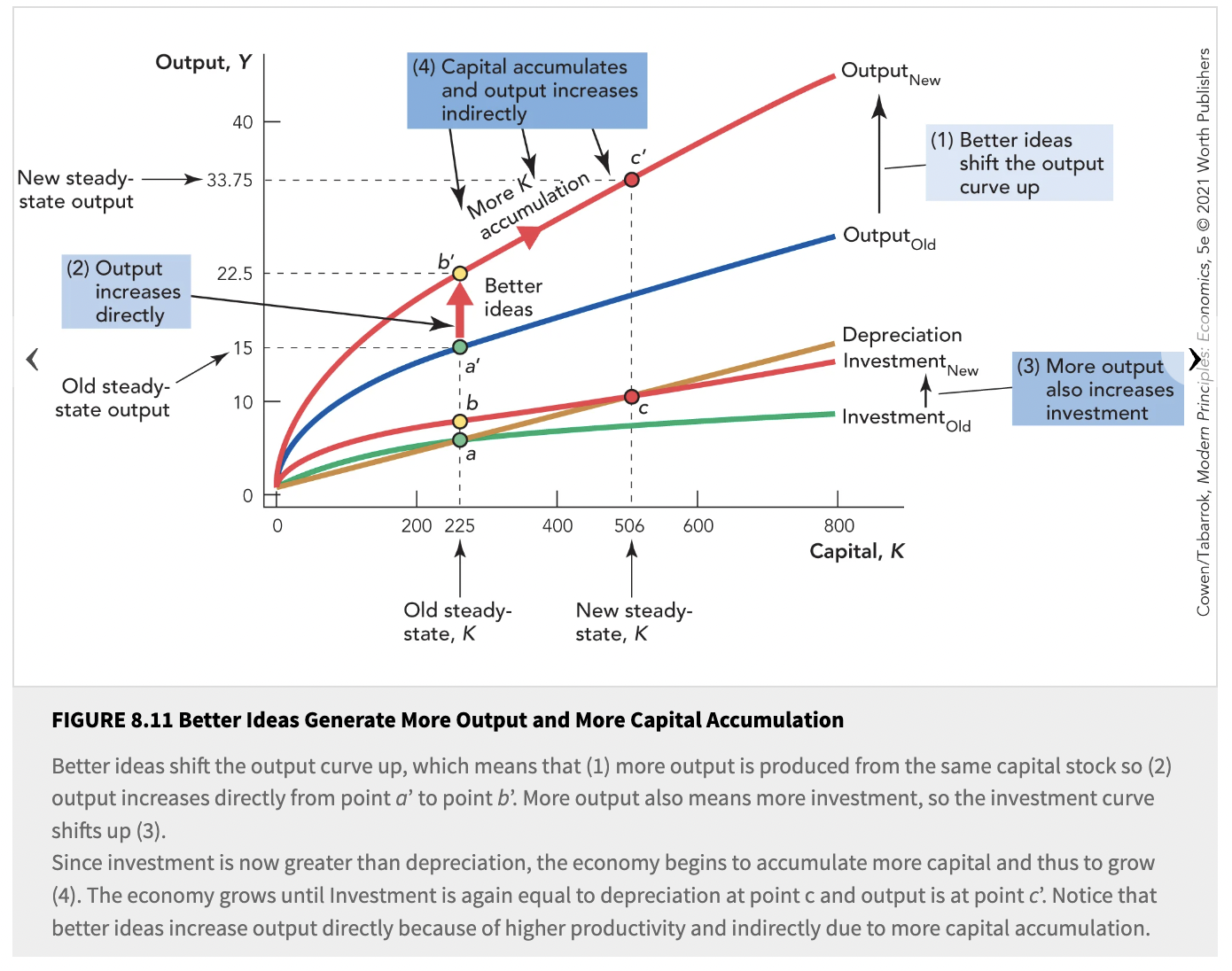
-Better ideas increase output directly and, by so doing, they increase capital accumulation indirectly.

- The process of economic growth is a continuous two-step process of better ideas and more capital accumulation.

The Economics of Ideas:

• Ideas can be freely shared by an unlimited number of people and they do not depreciate with greater use.
• Capital accumulation alone won’t create much growth in developed economies because these economies already have so much capital that investment must be used to replace a lot of depreciated capital every period. These countries must create new ideas in order to compete.

1. Ideas for increasing output are primarily researched, developed, and implemented by profit-seeking firms.
2. Ideas can be freely shared, but spillovers mean that ideas are underprovided.
3. Government has a role in improving the production of ideas.
4. The larger the market, the greater the incentive to research and develop new ideas.

• Economic growth requires institutions that encourage investment in physical capital, human capital, and technological knowledge (ideas).
• John Key: Invented the “flying shuttle” used in cotton weaving, the single most important invention launching the Industrial Revolution. Historically, entrepreneurs were often attacked as job destroyers, but recently are seen to be given support.
• Overall, the United States has a good cultural and commercial infrastructure for supporting new ideas and conversion into usable commercial products, including artistic innovation.

Patents:

• Many ideas are copied, such as the world’s first smartphone invented by IBM, in which other firms quickly coped the idea and IBM lost out in the race to innovate.
• People that do this are imitators, who often have lower costs because theyt do not have to pay development costs, and tend to drive innovators out of the market unless some barrier prevents quick imitation.
• Imitation often takes time which gives innovators the ability to recoup their investments. For example, the Apple iPad design had been copied by other firms, but before that, Apple was able to sell millions of iPads for high profits.
• However, Apple also relies on patents to protect its innovations. These delay imitations, allowing innovative firms a greater period of monopoly power. For example, Apple filed a patent in 2004, giving them the right to prevent other firms from copying its technology until 2024 and has patented the multipoint touchscreen aspect of the iPad.
• A majority of patented innovations are imitated within five years.

Spillovers, and Why there Aren’t Enough Good Ideas:

• The good aspect of imitation of spillovers is that ideas are nonrival. Nonrival is when one person’s consumption of the good does not limit another person’s consumption. Ideas can be freely shared.
• Since many ideas can be shared at low cost, they should be shared in order to maximize the benefit from an idea.
• Spillovers mean that the originator of an idea does not get all the benefits, and therefore ideas will be underprovided.
• While economists know that idea spillovers are good, they also know that spillovers mean that too few good ideas are produced in the first place.
• Example: A profit-maximizing firm invests in research and development so long as the private marginal benefit is greater than the marginal cost. Private investment occurs until point a, and spillovers mean that the social benefit of R7D exceeds the private benefit, so that the optimal social investment is found where the marginal social benefit just equals the marginal cost at point b.

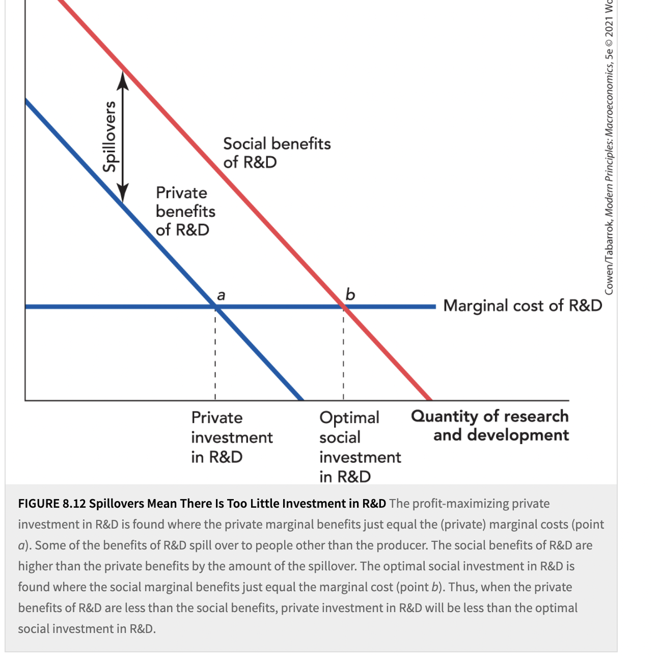
Government’s Role in the Production of New Ideas:

• Patents reduce spillovers and thus increase the incentive to produce new ideas, but they can also slow down the spread of new ideas. Prizes are another possibility.
• Example: In 2008, the U.S. Department of Energy offered $10 million to the first inventor to produce a new and more efficient lightbulb, and in 2011 Phillips claimed the prize with a 10-watt LED bulb that duplicated the light output of a 60-watt incandescent.
• An advantage of prizes is that the government does not have to decide in advance who can best solve a problem.
• Paying for innovation with a prize, rather than a patent also means that the idea can spread more rapidly.
• The government can also subsidize the production of new ideas. For example, in the graph, a subsidy or taxbreak to R&D expenditures will shift the private marginal cost of R&D curve down, increasing private investment.
• The argument for government subsidies is strongest when the spillovers are largest. For example, the founder of Dominos made a billion dollars producing pizza, whereas mathmeticians who create algorithms to be used all over the internet do not make nearly as much.
• The large spillovers to basic science suggest a role for government subsidies to universities, and most of the 1.3 million scientists who research and develop new products in the United States were trained in government-subsidized universities.

Market Size and Research and Development:

• The costs of developing drugs for rare and common ideases are the same, but the revenues are greater when the disease is more comon, so pharmeceutical companies concentrate on drugs for common diseases because larger markets mean more profits.
• Larger markets mean increased incentives to invest in research and development, more new drugs, and greater life expectancy.
• Many things (new computer chips, software, and chemicals) also require large R&D expenditures. AS many countries become wealthier, companies will increase their worldwide R&D (research and development) investments.

The Future of Economic Growth:

• Growth in per capita GDP was approximately zero from the dawn of civilization to about 1500 and 1760, doubled during the next hundred years, and increased even further during the nineteenth and twentieth centuries. Today, worldwide per capita GDP is growing by a little more than 3% per year.
• A (ideas ) = Population x Incentives x Ideas per hour
• The number of new ideas is a function of the number of people, the incentives to innovate. And the number of ideas per hour that each person has. This equation s a way of thinking about some of the key factors driving technological growth.
• In the world today, there are about 6 million scientists and engineers, 1.3 million of which come form the U.S. If many other nations were as wealthy as the U.S. and could devote more to R&D, there would be 5 times as many scientists and engineers. Thus, the world would get richer because of increased production of ideas.
• The population of the world is increasing and the incentives to innovate are also increasing.
• Consumers are richer and the world is becoming one giant integrated market because of trade; each of these factors boosts the incentives to innovate.
• The incentives to innovate also increase when innovators can profit from their investments without fear of expropriation.
• The least is known about the number of ideas per hour or how easy it is to come up with new ideas.
• In some places and times, knowledge grows by leaps and bounds, and in others it stagnates.
• When the law of diminishing returns is applied to ideas in general as well as to capital, then economic growth will be much slower.
• Two reasons for thinking that diminishing returns is not the usual state of affairs: many ideas make creating other ideas easier (for example, googling to find answers), and to think that the number of ideas per hour is not yet strongly diminishing comes from one of the pioneers of the economic ideas, Paul Romer. Romer points out that ideas for production are like recipes and the number of potential recipes in the universe is unimaginably vast (example tyhere are about 3,500 different sets of proportions for each choice of four elements, and 3,500 x 94,000 different recipes in total. If labs around the world evaluated 1,000 recipes each day, it would take nearly a million years to go through them all.
• Economic growth may be faster in the future than it has in the past due to the increasing population, increasing amount of scientists and engineers, and the incentives to invest in R&D are increasing because of globalization and increased wealth in developing countries such as China and India.
• Better institutions and more secure property rights are spreading throughout the world.

Takeaways:

• The Solow model is governed by the iron logic logic of diminishing returns. When capital stock is low, marginal product of capital is high and capital accumulates, leading to economic growth. But as capital accumulates, its marginal product declines, and growth stops.

The Solow Model tells us three important things about economic growth:

1. Countries devote a larger share of putput to investment will be wealthier. Wealthy countries have institutions that promote investment in physical capital, human capital, and technological knowledge.
2. Growth will be faster the farther away a country’s capital stock is from its steady-state value. This explains why German and Japanese economies were able to catch up to other advanced economies after WW2, why growth miracles oddur, and why poor countries grow faster than rich countries with similar levels of steady-state output.
3. The Solow model tells us that capital accumulation cannot explain long-run economic growth. Holding other things constant, the marginal product of physical and human capital will eventually diminish, thereby leaving the economy in a zero-growth steady state. If we want to explain long-run economic growth, we must explain why other things are not held constant.

• Ideas can be easily coped, meaning the originator won’t get the full benefits. Governments can play a role in supporting the production of new ideas by protecting intellectual property and subsidizing the production of new ideas when spillovers are most likely to be present.
• The non-rivalry of ideas, means that once an idea is created, we want it to be shared/coped as much as possible. There is a trade-off between providing appropriate incentives to produce new ideas and providing appropriate incentives to share new ideas.
• The larger the market, the greater the incentive to invest in research and development.

February 19th Notes:

Steady-state Level of Capital Continued:

• At some point, the capital stock reaches a level where every unit of investment is needed just to replace the capital that depreciates in that period
• When investment just covers capital depreciation, the capital stock stops growing
• When the capital stock stops growing, output stops growing as well.
• This is steady-state level of capital: The level where the capital stock is neither increasing nor decreasing. As the capital stock gets larger, the diminishing marginal product of capital menas output and investment will increase at a diminishing rate.
• Output = 2 times the square root of capital
• Investment is more than depreciation when capital stock grows, and the output next period becomes bigger.
• Investment equals depreciation when capital stock is constant, and output in the next period is constant.
• The steady-state stock of capital is where investment=depreciation. The level where the capital stock is neither increasing nor decreasing.
• Our capital stock reaches a steady-state level when Investment = Depreciation (Y=K).
• Y=f(K), so changes in the capital stock drive changes in output.
• Thus, when we reach a steady-state level of capital we also reach a steady-state level of output:
• Y*=f(K*)

:

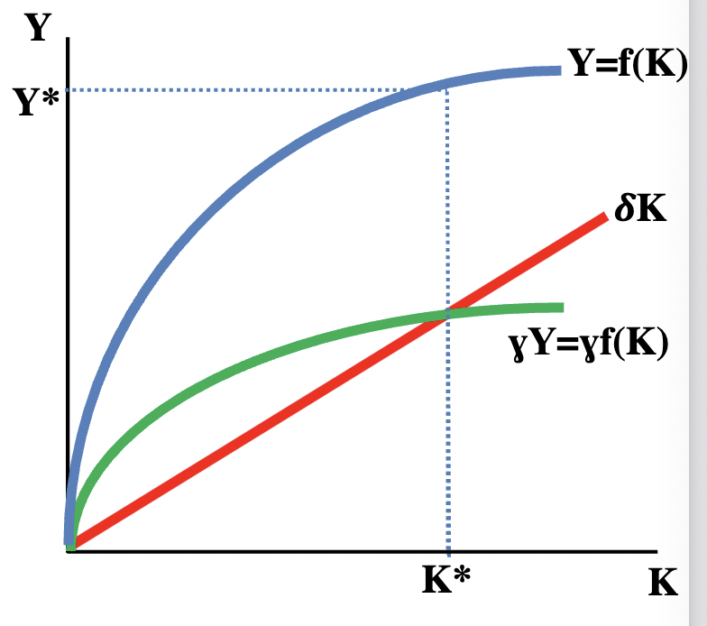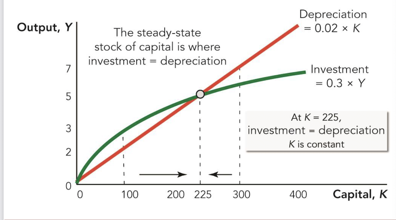
• When Investment > Depreciation, capital stock grows, and output next period is bigger
• When Investment = Depreciation, capital stock is constant and the output next period is constant
• When Investment < Depreciation, capital stock shrinks and output next period is smaller
• As the capital stock gets larger, investment increases but at a diminishing rate because the diminishing marginal product of capital.
• Depreciation increases with the capital stock at a linear (constant) rate.
• At some point, investment = depreciation
• This is the steady-state level of capital (where capital stock is neither increasing nor decreasing)

Catching Up Growth:

• The capital stock will grow as long as investment outpaces depreciation.
• Diminishing returns mean the difference between investment and depreciation decreases as (K/L) increases.
• Thus, growth in (K/L) and (Y/L) slows down
• Capital per worker (K/L) will eventually stop growing.
• Therefore, GDP per person will eventually stop growing as well.
• Long-run economic growth cannot be due to capital accumulation.
• The logic of diminishing returns applies to human capital as well.
• Changes in the capital stock drie output, so when Investment = Depreciation and K is at its steady-state level, then so is output.

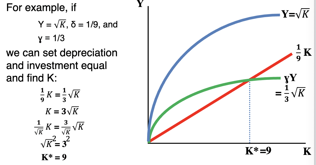
The Investment Rate:

• In the Solow model, a greater investment rate means more capital, which means more output.
• This increases a country’s steady-state level of GDP.
• Thus, the Solow model predicts that countries with higher rates of investment will be wealthier.
• The level of the capital stock determines the output level but not its growth rate, at least not in the very long run.
• Increased investment raises steady-state output

Investment and GDP

• GDP per capita is higher in countries with higher investment rates.

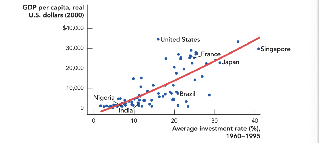
Conditional Convergence:

• The tendency–among countries with similar steady-state levels of output–for poorer countries to grow faster than richer countries and thus for poor and rich countries to converge in income.
• Suppose two countries with the same steady-state levels of capital (K*) and output (Y*)--one rich (high K) and one poor (low K).
• The poor country faces less depreciation and, thus, accumulates capital faster than the rich country.
• Each additional unit of capital will also have a higher marginal product for the capital-poor country than the capital-rich one.

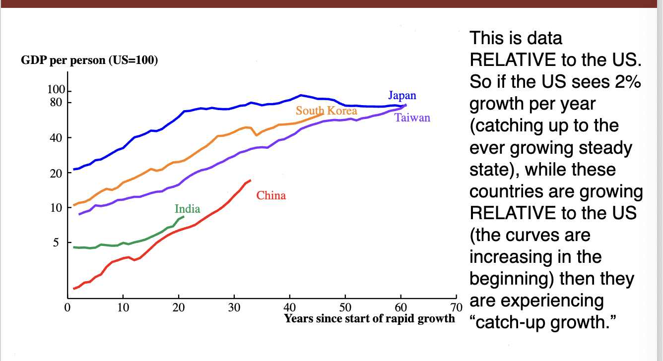
Cutting Edge Growth:

• The simplest form of the Solow model predicts zero economic growth in the long run.

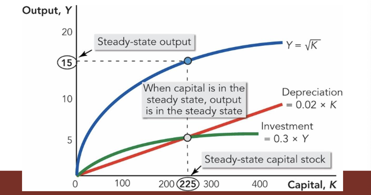
• The United states, however, has been growing steadily for more than 200 years.
• Better ideas can keep the economy growing even in the long run
• A computer today has about the same amount of silicon and labor input as 20 years ago, but today’s computer is much better–the difference is ideas.

K2=K1 + Investment-Depreciation (64 plus .25x2square root of 64)-0.5(64) .25 was the depreciation, .5 was investment and Y=2square root of K, K was 64.

Chapter 9 Notes:

• The Lehman bankruptcy shook the financial world, not simply because it was large but because Lehman Brotherd was an important financial intermediary, and institution that works to transform savings into investments.
• Lehman brothers failed because it had lost billions on buying and betting on mortgage securities. So had many other banks and financial institutions.
• Savings are necessary for capital accumulation, and the more capital an economy can invest, the greater is GDP per capita.
• Saving: Income that is not spent on consumption goods.
• Investment: The purchase of new capital goods;private spending on tools, plant, and equipment used to produce future output. It’s important to see that the way economists define investment is not the same as the way a stockbroker defines investment. Example: If Starbucks buys new espresso machines for its stores, that’s investment. If John buys stock in Stabucks, that is not investment in the economic sense but merely a transfer of ownership rights of already existing capital for a treatment of how individuals should allocate their funds.

The Supply of Savings:

• Economists have a good but imperfect understanding of what deterimes the supply of savings
• Individuals Want to Smooth Consumption: Consumption is high during your working years, but after retirement consumption drops precipitously–as a result, once you retire and your income falls, you must sell the nice car and give up the fancy lifestyle just to scrape by. But when retirement comes, consumption is greater than income as you spend your savings, or “dissave”.

• Economists say that Path B is “smoother” than Path A. The desire to smooth consumption over time is a reason to save and a reason to borrow.
• The consumption-smoothing theory of saving can tell us something important about AIDS, Africa, and economic growth.
• AIDS has dramatically reduced life expectancy in southern Africa.
• Fluctuations in income are another reason why people save.
• Individuals are Impatient: Another reason why people save, or fail to save, is their level of impatience. Most individuals prefer to consume now rather than later, so saving is not always easy. This is what economists call time preference. Impatience is reflected not just in savings but in any economic situation where people must compare costs and benefits over time. Crime is another economic activity with immediate benefits and future costs so it’s not surprising that criminals tend to be impatient people.
• Marketing and Psychological Factors: Marketing matters, even for savings. In businesses that use automatic enrollment, the savings plan participation rate was 25% higher than in the businesses in which employees needed to request a retirement account. In one firm, the default savings rate was 3% of salary. More than a quarter of the workers chose that as their savings rate, despite an employer guarantee of a dollar-for-dollar match on contributions up to 6% of salary. It’s surprising how some simple psychological changes, combine with effective marketing and promotion, can change how much people save for their retirement. Behavioral economics study how people can make decisions and how they can be helped to overcome biases in decision making.
• The Interest Rate: The quantity of savings also depends on the interest rate, namely how much savers are paid to save. Ex: If the interest rate is 5% per year, then $100 saved today returns $105 a year from now. If the interest rate is 10% per year, then $100 saved today returns $110 a year from now. Higher interest rates usually call forth more savings. The supply curve for savings has the interest rate on the vertical axis while other supply curves have had price on the vertical axis.

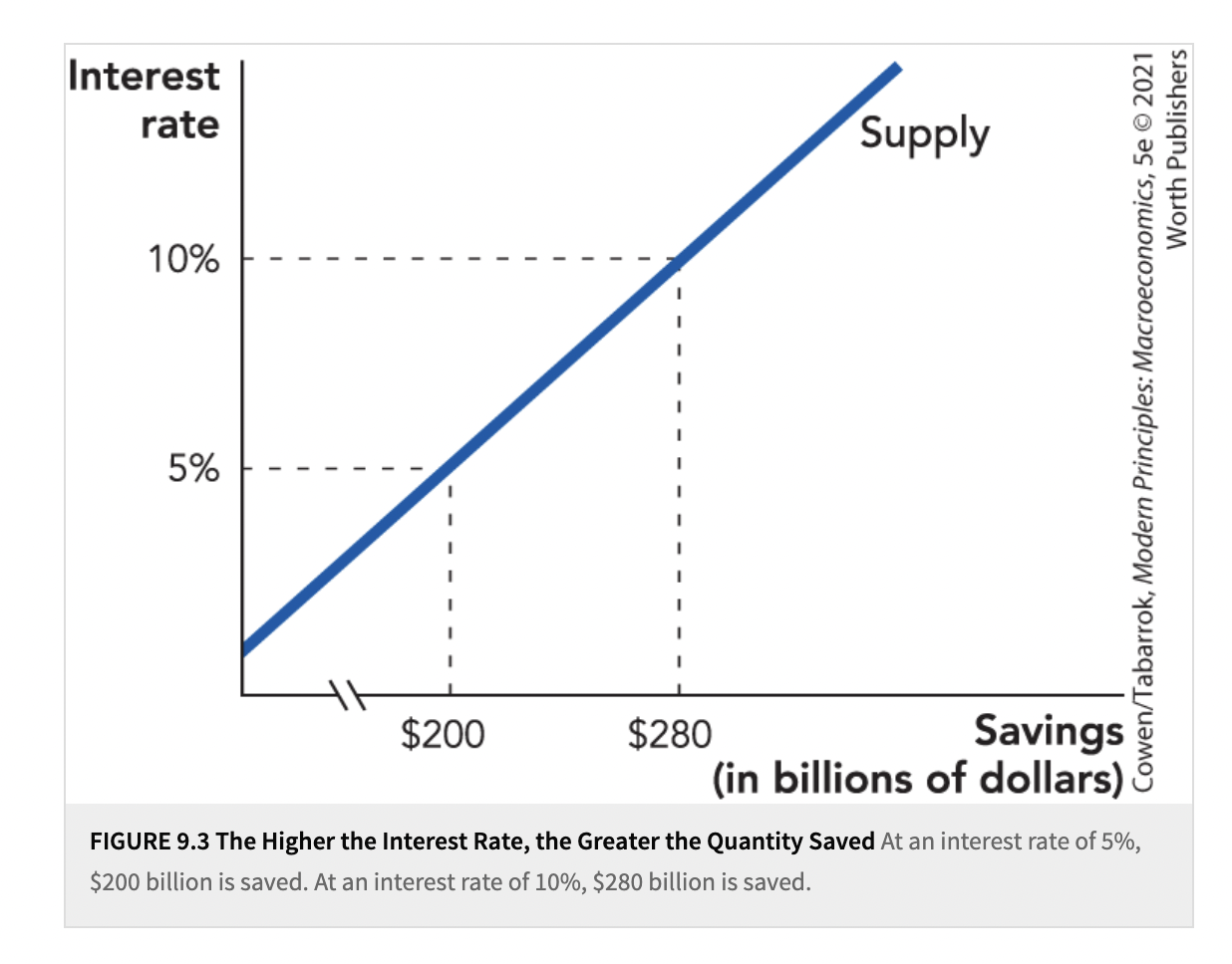
• Interest rate is a market price and it has the same properties of market prices that we discussed in the introductory chapters of this book.

The Demand to Borrow:

• Individuals Want to Smooth Consumption: Just as people save in order to smooth consumption, one reason people borrow is to smooth consumption. If tuition payments can be made over many years, as borrowing makes possible, the sacrifices are spread out and become less painful. A student who can borrow can move some of the sacrifices into future periods when the student has a job and regular income. Student borrowing is thus another example of how credit markets let people smooth their consumption over time. The “lifecycle” theory of savings puts the demand to borrow and save together. Governments also borrow for reasons much like consumers. They can buy to finance unusually large expenditures such as those required to pay for a war, or to pay for large investments such as the interstate highway system.

• Borrowing is Necessary to Finance Large Investments: Many new businesses can’t get under way at all without borrowing. Often the people with the best business ideas are not the people with the most savings, so people with good ideas borrow funds.
• Fred Smith: First laid out the idea for FedEc in an undergraduate paper for an economics class, and in order to be successful Smith began with 16 planes covering 25 cities using money he borrowed and also by selling part ownership of FedEc to venture capitalists, investors willing to accept risk in return for a stake in future profits.
• Businesses borrow to finance large projects
• The Interest Rate: The quantity of funds that people want to borrow depends on the cost of the loan, or the interest rate. Businesses, for example, borrow when they expect that the return on their investment will be greater than the cost of the loan. If the interest rate is 10%, businesses will borrow only if they expect that their investment will return more than 10%.

Equilibrium in the Market for Loanable Funds:

• Market for loanable funds: The market where suppliers of loanable funds (savers) trade with demanders of loanable funds (borrowers), thereby determining the equilibrium interest rate. In equilibrium, the quantity of funds supplied equals the quantity of funds demanded.

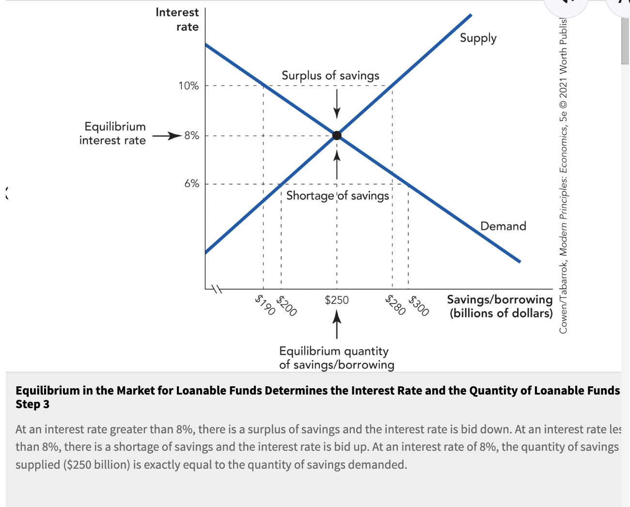
• The interest rate adjusts to equalize savings and borrowing in the same way and for the same reasons that the price of oil adjusts to balance the supply and demand for oil.
• Shifts in Supply and Demand: Changes in economic conditions will shift the supply or demand curve and change the equilibrium interest rate and the quantity of savings. An increase in the supply of savings is shown by shifting the supply curve to the right and down. An increase in the supply of savings causes the equilibrium interest rate to fall from 8% to 6% and the quantity of savings to increase from $250 billion to $300 billion.
• Example: South Korea. The shift in savings shows that South Korea’s increased savings were plowed into investment and one of the key drivers of economic growth is a high rate of investment and capital accumulation.

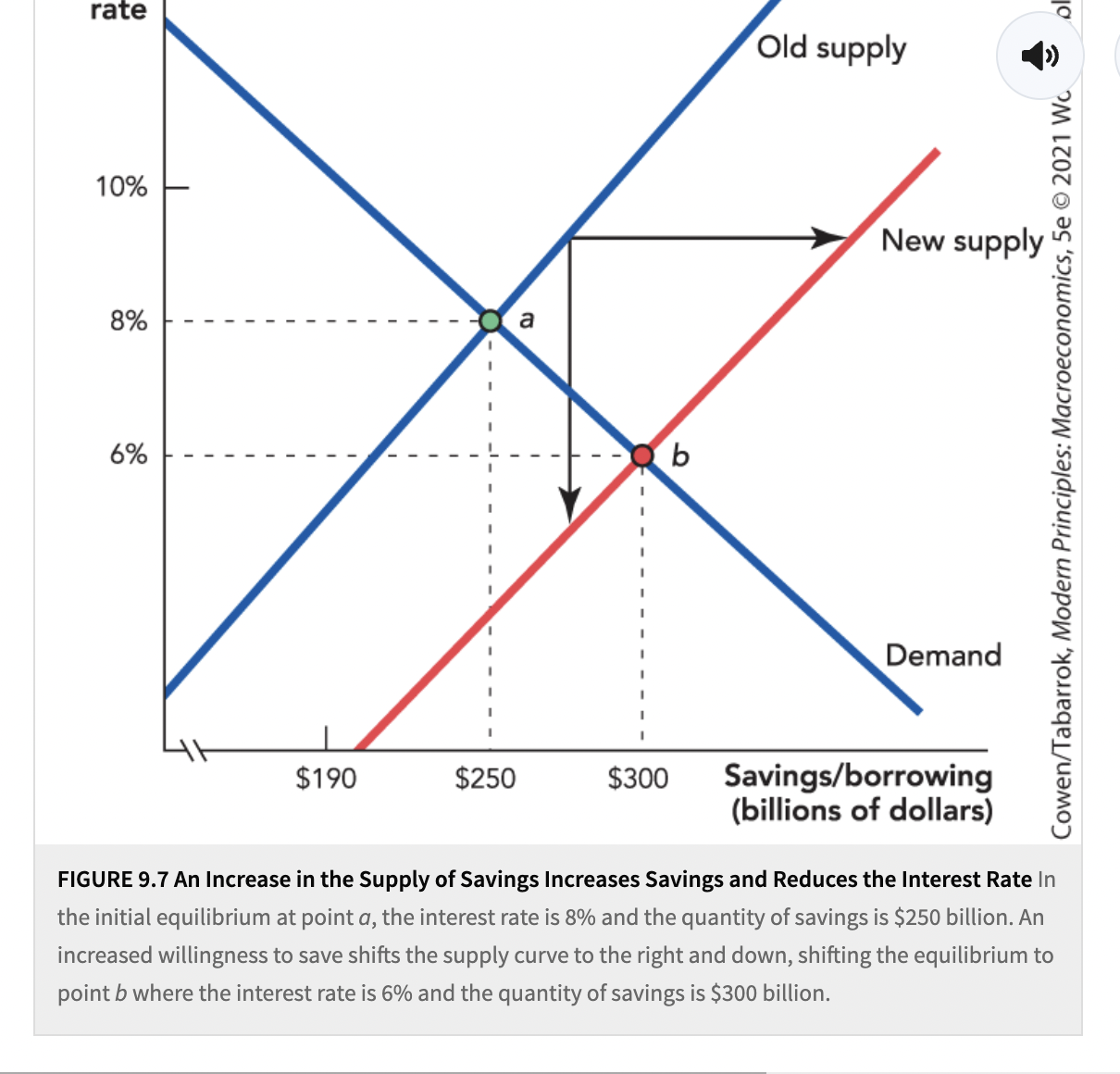
• A decrease in investment demand can itself help to spread and prolong a recession. A decrease in investment demand reduces the interest rate from 8% to 6% and the quantity of savings from $250 billion to $190 billion.

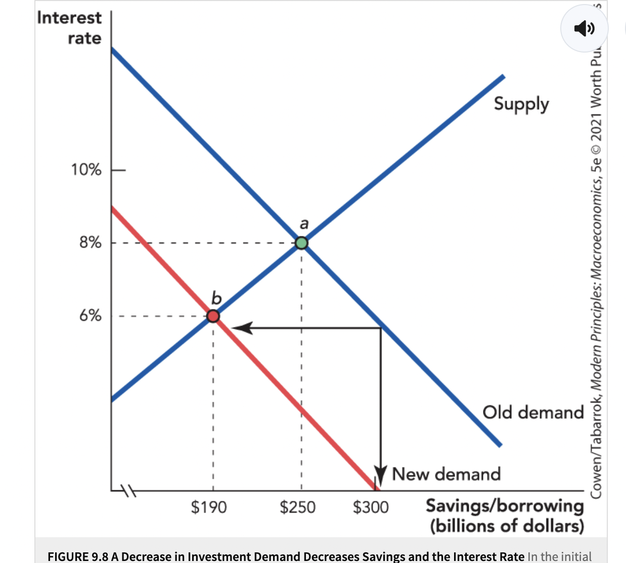
• An investment tax credit gives firms that invest in plants and equipment a tax break. The tax credit is usually temporary to encourage firms to invest quickly, when the recession is still in full force.

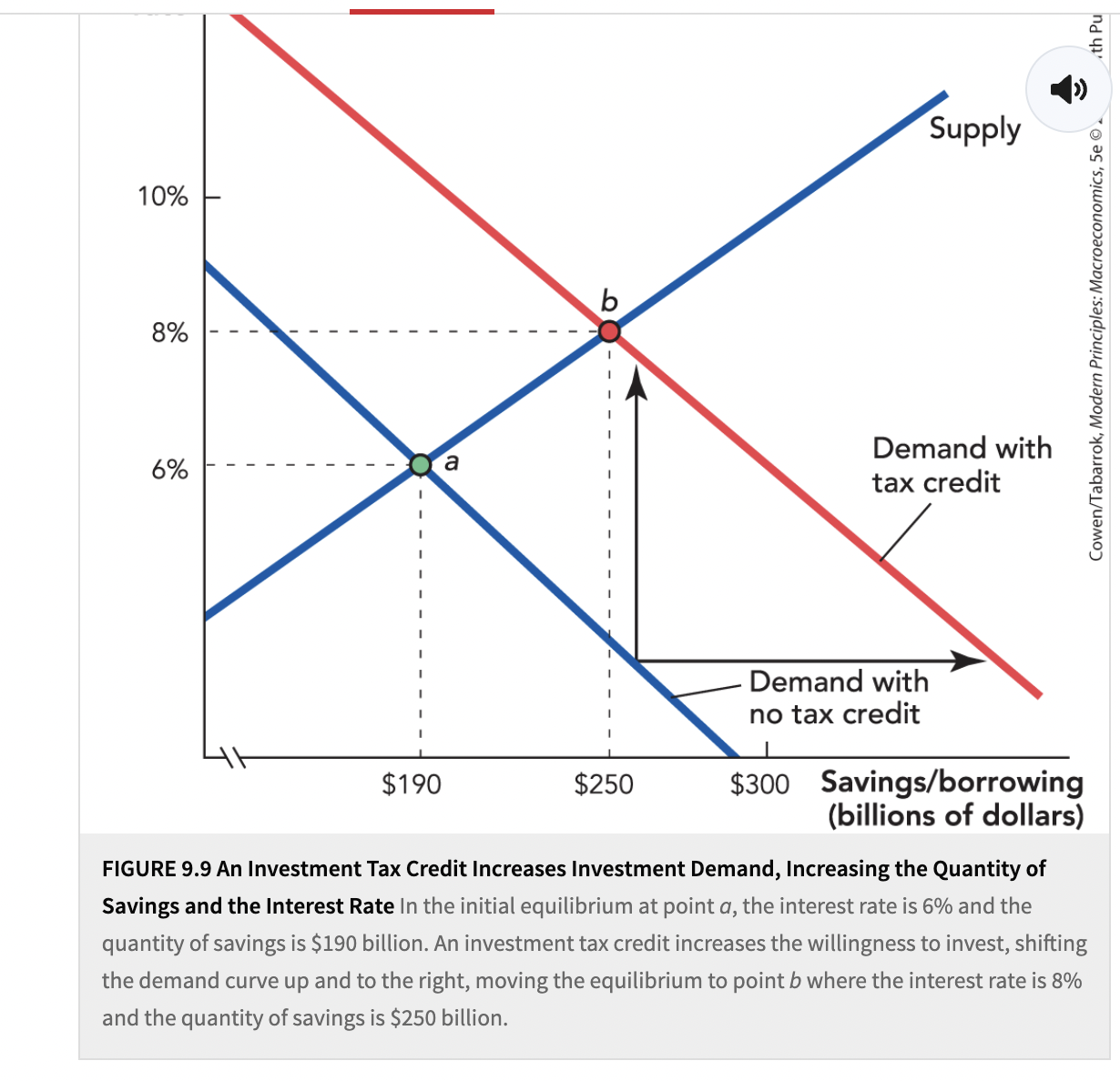
The Role of Intermediaries: Banks, Bonds, and Stock Markets:

• Equilibrium is brought about with the assistance of financial intermediaries such as banks, bond markets, and stock markets.
• Financial intermediaries reduce the costs of moving savings from savers to borrowers and helop mobilize savings toward productive uses
• Banks:
• Banks receive savings from many individuals, pay them interest, and then loan these funds to borrowers, charging them interest.
• When banks specialize, individual savers don’t have to evaluate which factories ought to be built or which businesses deserve to be supported.
• Banks coordinate lenders and minimize information costs and also play a role in the payments system.
• The Bond Market:;
• Investors can more easily find information about the firm and so they are willing to bypass the bank as an intermediary and lend to the company directly.
• When a member of the public lendsd money to a corporation, the corporation acknowledges its debt by issuing a bond. A bond is a sophisticated IOU that documents who owes how much and when payment must be made. It lists how much is owed to the bond’s owner and when payment must be made. In some cases money is owed on a single day, and in others, called coupon payments, are periodic payments that must be made in addition to a final payment.
• Example: The New York Central and Hudson River Railroad Company borrowed money in 1897 for which they issued bonds that promised the Central will pay the owner $1,000 in 1997. In addition, every six months until 1997, the Central promised to pay the owner $17.50. Central’s bond illustrates one of the advantages of bond finance–large sums of money can be raised now and invested in long-lived assets such as railroad track.
• Major bond issues are graded by agencies, AAA for example is the highest grade, and bonds rated less than BBB are sometimes referred to as “junk bonds”. If a risky company wishes to borrow money, it has to promise a higher rate of interest because lenders will demand to be compensated for a greater risk of default.
• Collateral: Something of value that helps to secure a loan; if the borrower defaults, ownership of the collateral transfers to the lender.
• Greater risk can reduce the supply of funds to the market as a whole. Governments can borrow money as well. As of 2016, the U.S. government owed about $14.4 trillion dollars to private borrowers. When the government borrows a lot of money, private consumption and investment can be crowded out.
• Crowded out: The decrease in private consumption and investment that occurs when government borrows more; also, the decrease in private spending that occurs when government increases spending.
• When the government borrows a great amount of money, the demand curve for loanable funds shifts right by that amount, increasing the interest rate. A higher interest rate draws an additional amount of savings into the market, meaning less consumption, and that some investments and other projects are no longer profitable, so at a higher interest rate, private borrowing falls. When the U.S. government borrows, it issues a variety of different bonds.
• Bond Prices and Interest Rates:
• Rate of return for a zero-coupon bond = Face value - Price/Price x 100
• If interest rate rises the price of the bond falls. Equally risky assets must have the same rate of return. If they didn’t, no one would buy the asset with the lower rate of return and the price of that asset would fall until the rate of return was competitive with other investments.
• Arbitrage principle: The practice of taking advantage of price differences for the same good in different markets by buying low in one market and selling high in another market. Interest rates and bond pieces move in opposite directions. (buy low-sell high)
• The Stock Market:
• Stocks are shares of ownership in a corporation. Just as businesses fund their activities by taking out bank loans and selling bonds, they also issue shares of stock. Owners have a claim to the firm’s profits. If profits are high, shareholders benefit, they benefit directly if the firm pays out its profits in dividends or indirectly if the firm reinvests its profits in a way that increases the value of the stock.
• Initial public offering: The first instance of a corporation selling stock to the public in order to raise capital.
• Simply buying and selling existing shares of stock does not increase net investment in the economy. Example: Google sold $1.67 billion worth of stock in an IPO in 2004, which helped to fund new investments and pay for research and development. The big payoff was a reward for creating the company and making the early and risky necessary investments to get Google off the ground. It also let the founder diversify and encourages innovation.
• IPO: A first-time sale of a firm’s stock to the market.

What Happens When Intermediation Fails?

• The bridge between savers and borrowers can be broken in many ways, including insecure property rights, inflation and controls on interest rates, politicized lending, and massive bank failures and panics
• These problems can break the bridge by: reducing the supply of savings, raising the cost of intermediation, and reducing the effectiveness of lending.

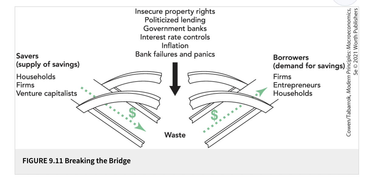
• Insecure Property Rights: Some governments do not offer secure property rights to savers. Ex:During Argentine’s 2001 financial crisis, the government partially froze bank accounts for a year, which meant that banks went under and citizens lost their bank-based savings.
• If individuals expect that contracts will be broken, they will be reluctant to invest in stock markets as well. For example, the Russian government often doesn’t respect the rights of minority shareholders and at times it has confiscated or restricted the value of their shareholdings. Law is on one side of the equation, but custom and informal trust are another. In a healthy economy, shareholders except that managers are interested in building their long-run reputations rather than ripping off the company at every possible opportunity.
• Controls on Interest Rates:
• Price controls on interest rates also cause the loanable funds market to malfunction. Consider a maximum ceiling on the interest rate that can be charged on a loan. Sometimes economists call these ceilings “usury laws”. A ceiling on interest rates creates a shortage of savings. At the artificially low price, there is a shortage of credit, and many people who wish to borrow at the controlled interest rate cannot do so. Investment, which is determined by the supply of savings will fall below what it would be at the market equilibrium.

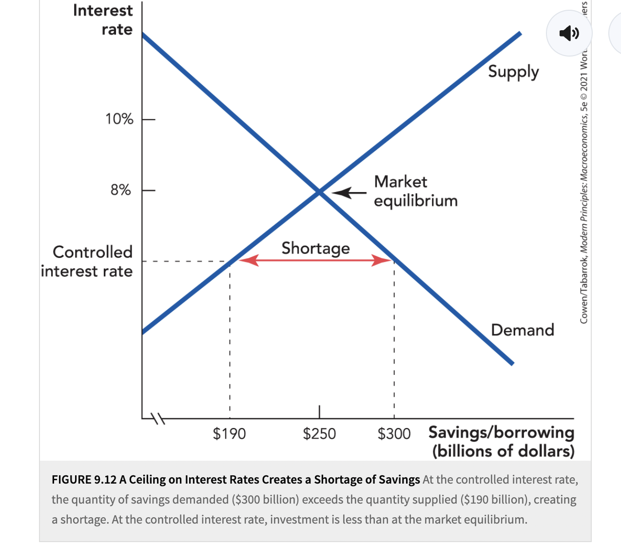
• Politicized Lending and Government-Owned Banks: Government-owned banks are useful to authoritarian regimes that use the banks to direct capital to political supproters. In a stuyd by economists Rafael La Porta, Florencio Lopez-de Silanes, and Andrei Shleifer found that the larger the fraction of government-owned banks a country had in 1970, the slower the growth in per capita GDP and productivity over the next several decades.
• Bank Failures and Panics: Systematic problems in the banking system usually lead to large-scale economic crises. During the Great Depression, bank failures were followed by a rash of small business failures. Authors Milton Friedman and Anna Schwartz argued that the Great Depression was brought about, in part, because the Federal Reserve–the U.S. central bank that is charged with overseeing the general health of the banking industry–failed in its job to prevent widespread bank failures.

The Financial Crists of 2007-2008:

• Bernanke: Chairman of the Federal Reserve between 2006-2014, and had to face the worst intermediation crisis since the Great Depression.
• Lending: In the years leading up to the financial crisis, Americans borrowed more than every before, especially in the closely related sectors of home mortgages and banking. The difference between the value of a house and the unpaid amount on the mortgage is called the buyer’s equity or owner’s equity. At the height of the housing boom in 2006, 17% of mortgages were made with 0% down. If house price rose, they could borrow more or sell at a profit.
• Leverage ratio: The ratio of debt to equity, D/E (example: If a buyer of a $400,000 house borrows $320,000 and spends $80,000 of her own savings, then her leverage ratio is 4=$320,000/$80,000)
• Home buyers weren’t the only ones leveraging more, so were banks (Ex: Lehman brothers had assets worth hundreds of billions of dollars but it had borrowed hundreds of billions of dollars to but those assets. Their leverage ratio was around 20, which is pretty high, and if their assets were to fall even by 10%, it would make Lehman insolvent).
• Insolvent: A bank or institution whose liabilities are greater in value than its assets.
• When times are good, leverage makes everything better, which is why banks may want a high leverage ratio. When things go poorly, managers also had limited downside risk, so even when Lehman went bankrupt, the managers lost some money but still ended up being very rich.
• Securitization: Sometimes loans are bundled together and sold on the market as financial assets. Banks may wish to securtize their loans for several reasons, because they may get more liquid cash and it makes their balance sheet safer, and the securitized assets can be held as investments by institutions with a long-term perspective, such as pension funds.
• Once assets are securitized, the revenue streams from them can be sliced and diced and sold in all manner of ways.
• The increased ability to sell mortgages around the world was good for American home buyers because it kept interest rates low and it seemed good for investors who thought they were buying safe and secure assets. When housing prices started to fall dramatically, many began to default on their mortgages. Buyers had only a little equity in their homes so as house prices fell they quickly came to owe more on their mortgage than their house was worth and many chose to default.
• The Shadow Banking System: Has become a common term since the financial crisis.
• In a commercial bank the money comes from depositors, and in an investment bank the money comes from the investors. Deposits are guaranteed but investments are not, so investors are more prone to panic and withdraw their short-term funding in times of crisis. The shadow banking system got its name because it grew up in the shadow of the traditional banking system and for a long time most regulators and policymakers were unaware of its importance.
• Fire Sales: The financial crisis can be understood as a run on the shadow banking system similar in many aspects to bank runs during the Great Depresssion.
• The short-term loans disappear most quickly because they are rolled over on a very frequent basis–sometimes nightly.
• Without short-term loans, the investment bank no longer has enough operating funds and it is forced to sell off assets quickly in what is often called a “fire sale,”. Ex: Imagine there are three financial assets, A, B, and C, and suppose that an external event, such as a fall in housing prices, causes a fall in the price of A. The fall causes people to worry, and the worried lenders begin to demand greater collateral on their loans. With less money, the bank is forced to sell asset A, and some holdings ofo B and C. The price ofo B and C are pushed down, and lenders fear the intermediaries may go bankrupt, so even more intermediaries must sell assets and cut back on lending, and so the problem gets worse. When intermediaries fail, credit dries up ad the firms that were relying on that credit also begin to fail, adding another vicious cycle to the mix. The fire sale problem was a major issue in the 2008-2009 recession. This occurred for Lehman, which caused short-term lenders to flee from Lehman, triggering its financial meltdown.
• Shadow banks in particular relied on short-term funding, which was not guaranteed, so lenders withdrew their short-term funding, leading short-term banks to fall victim to the fire of the sale.
• New financial regulations are regulating these financial intermediaries in ways similar to traditional banks.

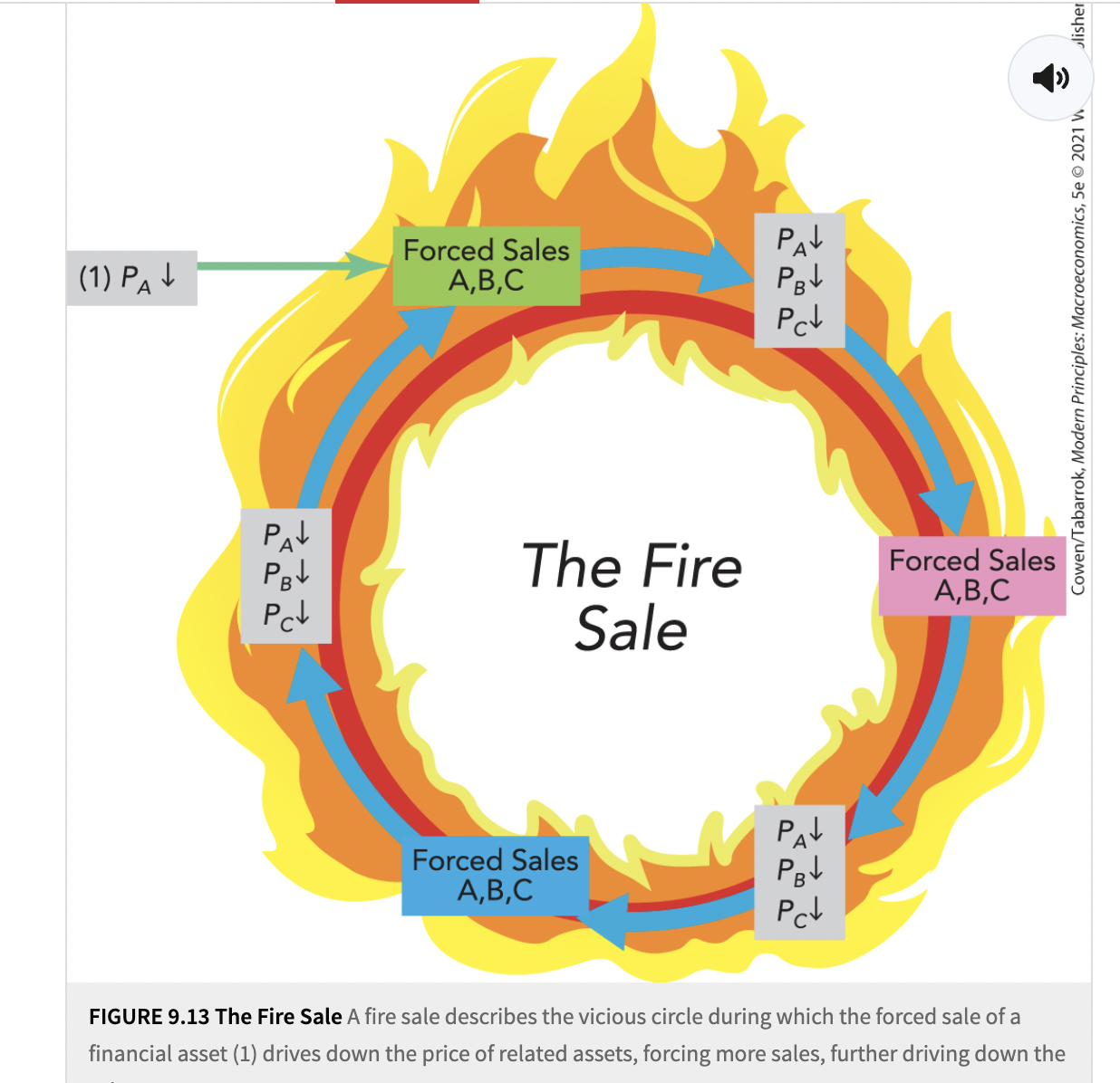
Takeaways:

• Borrowing helps agents to smooth their consumption streams
• Financial intermediaries also collect savings evaluate investments, and diversify risk.
• Without effective financial intermediation, an economy will end up adrift.

February 21st Notes:

The Limits of Capital:

• The Solow Model

The Economics of Ideas:

1. Ideas for increasing output are primarily researched, developed, and implemented by profit-seeking firms.
2. Ideas can be freely shared, but spillovers mean that ideas are underprovided
3. Government has a role in improving the production of ideas.
4. The larger the market, the greater the incentive to research and develop new ideas.

Research for Profit:

• The incentives created by institutions shape the generation of technological knowledge.
• These institutions include:

- A setting that helps innovators to connect with capitalists

- Intellectual property rights

- A high-quality educational system

• The United States has a very good cultural and commercial infrastructure for supporting new ideas and their commercialization

Techological Spillovers:

• Technological knowledge and other ideas are non-revalrous

- That is, one person’s consumption of a good does not limit another person’s consumption.

- Thus, one person’s innovative idea can benefit all members of a society

Patents

• New processes, products, and methods can be copied by competitors
• Imitators have lower costs and tend to drive innovators out of the market unless barriers prevent quick imitation
• Patents give innovators temporary monopoly rights, typically 20 years.
• Patents increase the incentive to develop new products, but they also increase monopoly power
• Monopoly power raises prices and slows the spread of innovations throughout the economy
• The trade-off between creating incentives for R&D while avoiding too much monopoly power is one of the trickist in economic policy
• Even with patents, ideas tend to spill over and benefit other firms and consumers
• Since ideas are non-rivalrous and many can be shared at low cost, society will be better off if they are shared
• However, if the originator doesn’t get enough of the benefits, ideas will be underprovided
• Economists know that idea spillovers are good; they also know that spillovers mean that too few good ideas are produced in the first place.

Technological Spillovers and Research for Profit:

• To help align incentives, governments create patents, which give innovators temporary monopoly rights, typically 20 years.
• The trade-off between creating incentives for R&D

Government’s Role:

• The government can increase the incentive to produce new ideas through patents
• The government can also encourage the production of new ideas through subsidies or tax breaks
• Universities train scientists who research and develop new products
• The large spillovers to basic science suggest a role for government subsidies to universities.

The Future of Economic Growth:

• The number of people in the world is increasing
• As the world gets richer, the number of people whose job it is to produce new ideas is increasing
• Because of spillovers, these ideas will benefit everyone
• Increased consumer wealth and integrated markets boost the incentive to innovate
• Economic growth might be even faster in the future than it has been in the past

Takeaways:

• The Solow model tells us that:

- Countries that devote a larger share of output to investment will be wealthier

- Growth will be faster the further away a country’s capital stock is from its steady-state

- Capital accumulation cannot explain long-run economic growth

Chapter 9 Lecture Notes:

• Y=C+I+G+NX
• The more an economy can invest as new capital, the greater its per capita GDP will be
• Saving: Income that is not spend on consumption goods
• Investment: The purchase of new capital goods
• Savers and investors are often different people, linked by the loanable funds market
• Connecting savers and borrowers increases gains from trade and smooths economic growth (Savers include supply of savings, ex: households, firms, venture capitalists) (Borrowers include demand for savings ex: firms, entrepreneurs, households)

The Supply of Savings:

• Four major factors determine the supply of savings:

- Smoothing consumption

- Impatience

- Marketing and psychological factors

- Interest rates

Consumption Smoothing:

• If you consume what you earn every year, consumption is high during your working years.
• After retirement, consumption would drop precipitously

- Since we enjoy a declining marginal utility of consumption, this will leave us worse off overall than if we consumed a constant amount

• You can smooth your consumption by saving during the working years and dissaving during the retirement years
• Saving also builds a cusion for unemploymen t or unexpected health problems
• Remember the rational rule for consumers

- People will consume more today if the marginal benefit of a dollar of consumption today is greater or equal to the marginal benefit of spending a dollar-plus-interest in they future.

• Thus, rational consumers practice consumption smoothing

- That is, they maintain a steady or smooth path or of consumption spending over time

• The permanent income hypothesis holds that you choose how much to consume based on your permanent income (your best estimate of your long-term average income) rather than your current income

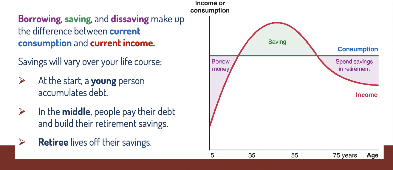
Individuals Are Impatient:

• Most individuals exhibit some degree of time preference, or the desire to have goods and services rather than later (all else being equal)

- Criminals, addicts, alcholocs, and smokers all tend to discount the future more heavily.

• Individuals’ time-preference will determine how they weigh the marginal benefit consumption today vs. the marginal benefit of future consumption
• The more impatient a person is, the more likely that person’s savings rate will be low

Marketing and Psychological Factors:

• Simple psychological changes, combined with effective marketing and promotion, can change how much people save
• Individuals save more if saving is presented as the natural or default alternative

- The retirement savings plan participation rate was 25% higher in businesses that used automatic enrollment rather than an opt-in feature

The default also mattered for how much was saved.

The Interest Rate

• The supply curve for loanable funds follows the law of supply
• The higher the interest rate, the greater the quantity saved
• The interest rate is the cost of consuming today rather than saving to consume in the future
• If you get interest on your savings, the future value of your account will equal the present value of your account will equal the present value of your account multiplied by (1+interest rate):
• FV = PV (1+r)
• Thus, the higher the interest rate, the greater the opportunity cost of consuming an amount today rather than saving it and lending it out

The Demand to Borrow:

• Three major factors to determine the demand to borrow:

- Consumption smoothing and human capital investment

- Business investment

- Interest rates

If someone never saves or borrows their income will equal consumption

Consumption Smoothing:

• Workers can smooth consumption over their lifetimes by borrowing, saving, and dissaving
• Many young people borrow to enjoy a decent standard of living while investing in their educations.
• Borrowing moves some sacrifices into future periods when students have a job

Investment:

• Often the people with the best business ideas are not the people with the most savings
• Businesses borrow to finance large projects
• The ability to borrow greatly increases the ability to invest
• Higher investment increases the standard of living and the rate of economic growth

Interest Rates:

• The demand curve for loanable funds follows the law of demand
• The lower the interest rate, the greater the quantity of funds demanded
• A higher interest rate raises the cost of a loan

Savings, Investment, and the Market for Loanable Funds:

• Economists define a market as a group of buyers and sellers of a particular good or service
• The market for loanable funds is the market where suppliers of loanable funds trade with demanders of loanavle funds
• Trading in the market for loanable funds determines the equilibrium interest rate

Equilibrium in the Market for Loanable Funds:

• In equilibrium, the quantity of funds supplied equals the quantity of funds demanded.
• The interest rate adjusts to equalize savings and borrowing

Shifts in Supply and Demand:

• As in any other market, changes in economic conditions will shift the supply or demand curve
• The shift will change the equilibrium interest rate and quantity of savings

Greater Savings and Borrowing:

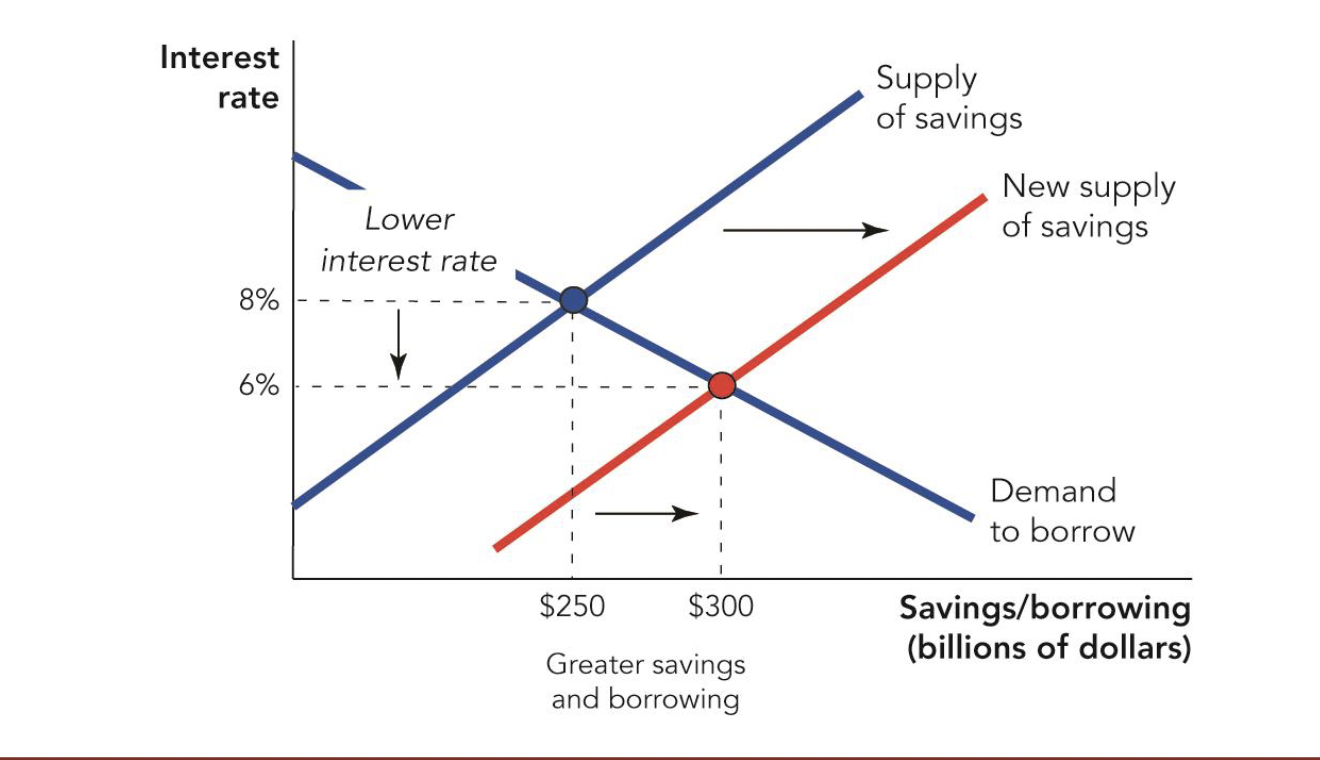
Investors Become Less Optimistic

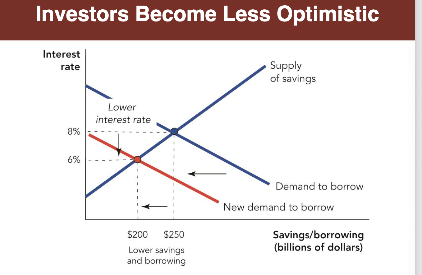
The Role of Intermediaries:

• Equilibrium in the market for loanable funds does not come about automatically

- Savers move their capital to find the highest returns

- Entrepreneurs must find the right investments and the right loans

- And financial intermediaries like banks, bond markets, and stock markets reduce the costs of moving savings from savers to borrowers and investors.

Banks:

• Banks receive savings from many individuals/firms and pay them interest
• They loan these funds to borrowers, charging them interest
• Banks profit by charging more interest on loans than they pay on savings
• But banks still bring us as close to equilibrium as possible
• Banks earn their profits by providing services such as evaluating investments and spreading risk
• By specializing in loan evaluations, banks are better able to decide which business ideas make sense:

- It would be wasteful if every saver spent time evaluating the same business

- Banks coordinate lenders and minimize information costs.

• Banks spread default risk across many lenders
• Banks also play a role in the payments system
• Banks also earn their profits by providing services such as evaluating investments and spreading risk
• By specializing in loan evaluations, banks are better able to decide which business ideas make sense:

- It would be wasteful if every saver spent time evaluating the same business

- Banks coordinate lenders and minimize information costs

• Banks spread default risk across many lenders
• Banks also play a role in the payments system

The Bond Market:

• Savers can easily find information about large, well-known corporations, allowing them to bypass banks and lend to these companies directly

- A corporation can thus borrow money by issuing a bond, or corporate IOU.

- A bond contract promises that the corporation will pay back what it borrowed (principal) with interest according to a specified schedule

• Bonds are a way to raise a large sum of money for long-lived assets, and they can be paid back over a long period of time.
• All bonds involve default risk, or the risk that the borrower will not pay back the loan

- A risky company has to pay higher interest to compensate lenders for greater default risk.

- But bondholders have priority in bankruptcy hearings, giving them additional security vis-a-vis stockholders.

- Thus, bonds came with collateral, or something of value that, by agreement, becomes the property of the lender if the borrower defaults.

• Interest rates differ depending on the borrower, repayment time, amount of the loan, type of collateral, and many other features.

U.S. Government Bonds:

• Treasury securities are desirable because they are easy to buy and sell, and the U.S. government is unlikely to default
• T-bonds: 30-year bonds; they pay interest every 6 months.
• T-notes: Maturities range from 2 to 10 years; they pay interest every 6 months.
• T-bills: Maturities range from a few days to 26 weeks; they pay only at maturity.
• Zero-coupon bonds: “Discount bonds”; they pay only at maturity.Rate of return depends on what price you pay for it depending on the face value.

Government Borrowing and the Bond Market:

• We can see crowding out, where the government borrowing more leads to a decrease in private consumption and investment

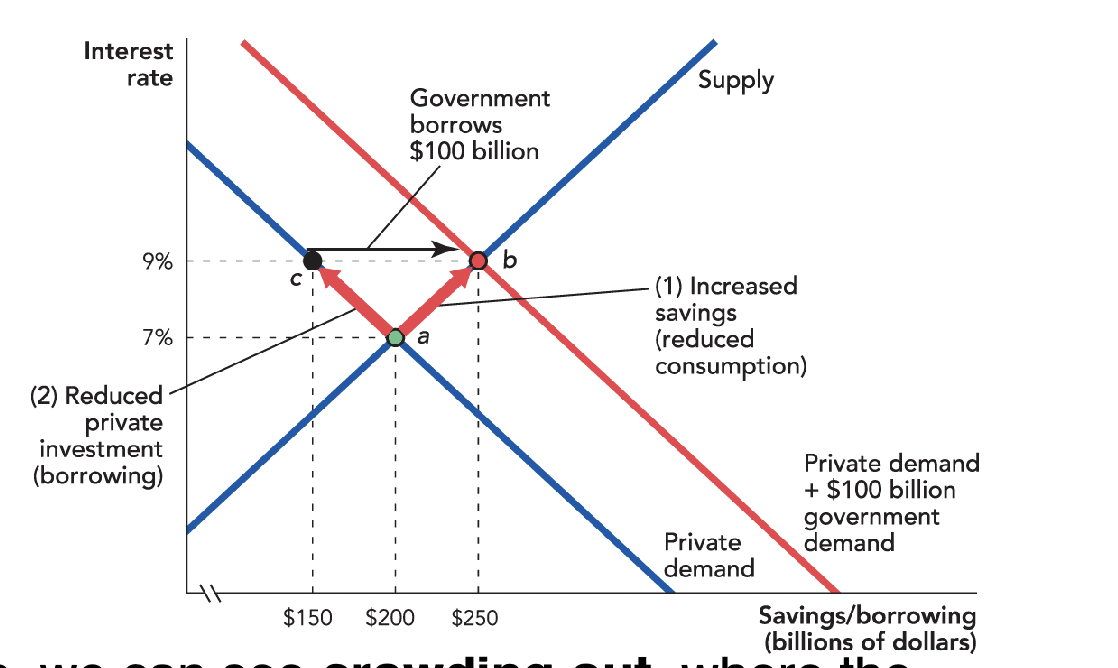
• Summary of previous graphs:

- A $100 billion increase in government borrowing crowds out private consumption and investment.

- Total and private investment equaled $200 billion in the original equilibrium

- Total investment equals $250 billion in the new equilibrium, but private investment equals $150 billion. Public investment due to government borrowing accounts for the additional $100 billion.

- Private consumption decreases and savings increases due to the higher interest rate

- Private investment decreases by $50 due to increased government borrowing.

Bond Prices and Interest Rates:

• Equally risky assets must have the same rate of return.
• If they didn’t no one would buy the asset with the lower rate of return.
• The price would fall until the rate of return was competitive with other investments.
• This is called an arbitrage principle:

- Arbitrage is the buying and selling of equivalent assets to earn a profit from buying low and selling high; arbitrage ensures that equally risky assets earn equal returns

• If you get interest on your savings, the future value of your account will equal the present value of your account multiplied by (1+the interest rate): FV = PV (1+r)
• We can rearrange this equation to find the present value of a future payment: PV = FV/1+r
• The value of a bond at matury is called the face value (similar to future value
• The relationship between a bond’s face value and its current price will affect the rate of return you earn from holding a bond.
• The rate of return, or implied interest rate, on a zero coupon bond can be calculated as: Rate of return = FV-Price/Price x 100
• This tells us that when interest rates go up, the value of existing bonds fall, because you can now get a better return on new debt (the opportunity cost has gone up)
• Interest rates and bond prices move in opposite directions.
• When interest rates go up, bond prices fall; when interest rates go down, bond prices rise.
• This tells us that in addition to facing default risk, people who buy bonds also face interest rate risk
• The value of a bond at maturity is called the face value. The rate of return, or implied interest rate, on a zero-coupon bond can be calculated as: Rate of return =
  FV-Price/Price x 100
• If you pay $909 for a 1-year bond with a face value of $1,000: Rate of return = 1,000-909/909 x 100 = 10%

The Stock Market:

• Businesses can fund their activities by issuing stock, certificates or shares of ownership in a corporation
• Stocks are traded on organized markets called stock exchanges.
• Buying and selling existing shares of stock does not increase net investment in the economy

- It merely transfers ownership of existing assets

• Though buying and selling stock itself does not increase net investment in the economy, a firm first selling shares to the public often funds an investment with the proceeds.

- We call the first time a firm sells stock to the public its initial public offering (IPO).

• Stock markets encourage investment and growth by helping firms to raise funds to invest in new capital.

Stocks vs. Bonds:

Bonds:

• Specified future interest payments
• First in line to get paid if the company goes bankrupt
• No rights to help control the company

Stocks:

• Uncertain future dividends; depending on how well the company is doing
• Last in line to get paid if the company goes bust
• Shareholders have a vote in how the company is run

When Intermediation Fails:

• The bridge betweemn savers and borrowers can be broken in many ways

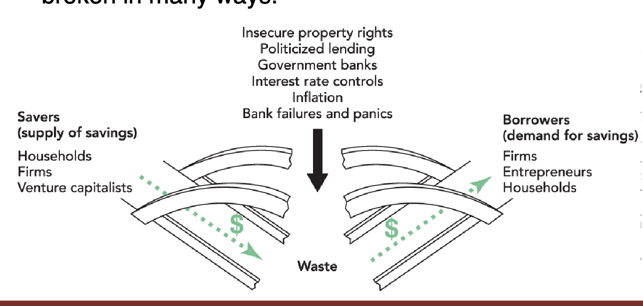
Chapter 9 Note-February 26th:

Self-Check:

1. With a 7% interest rate, we would expect the current price of a zero-coupon bond paying $5,000 in a year to be:
2. A zero-coupon bond will pay its holder $1,000 in a year. If its current price is stable at $960, then the interest rate on similarly risky loans must be:

Takeaways:

• Saving and borrowing allows individuals, firms, and governments to smooth their consumption over time
• Financial intermediaries bridge the gap between savers and borrowers
• Financial intermediaries also collect savings, evaluate investments, diversify risk, and help finance new and innovative ideas

Lecture-Exam Review Chapter 8:

Catching Up and Conditional Convergence:

• Each additional unit of capital→higher marginal product
• Cutting-Edge growth: In the developed stage, but increases output due to technological advancements and ideas

The Solow Model:

• The square root of capital is the output
• Capital also depreciates at a certain depreciation rate, and to find the depreciation rate you wound only use K (delta times K) To find delta, you would use slope
• To find capital stock of next year it would equal out current capital stock plus current investment minus current depreciation:
• Kt+1=Kt+Yyt=DKt
• Kt+1=Kt+yF(Kt)-DKt

ECON 2105 Unit 3 Notes:

Chapter 11 Notes:

• Someone who is unemployed is counted as unemployed only if they are willing and able to work but cannot find a job.
• In June 2017, for example, there were 7.0 million unemployed people in the United States and 153.2 million employed people. Together, the employed and the unemployed make up the labor force of 160.2 million (7+153.2)
• The unemployment rate is the percentage of the labor force without a job: unemployed/unemployed + employed x 100=Unemployed/Labor force x 100
• In June 2017, the unemployment rate was 4.4%: 7 million/7 million + 153.2 million x 100 = 7/160.2 x 100 = 4.4%
• Labor Force Participation Rate: The percentage of adults in the labor force.
• Discouraged workers: Jobless individuals who have given up looking for work but who would still like to find a job. The number of discouraged workers in the United States is small relative to the number of unemployed increases the unemployment rate only modestly.
• The unemployment rate doesn’t measure the quality of the jobs people take or how well workers are matched to their jobs.
• Unemployment rate: A Bureau of Labor Statistics measure that includes part-time workers who would rather have a full-time position and people who would like to work but have given up looking for a job. This includes part-time workers who would rather have a full-time position and also people who would like to work but have given up looking for a job
• Economists distinguish three types of unemployment: frictional, structural, and cyclical.

Frictional Unemployment:

• Frictional unemployment is short-term unemployment caused by the ordinary difficulties of matching employee to employer
• Scarcity of information is one of the causes of frictional unemployment because workers don’t know all the job opportunities available to them, and employers do not know all the available candidates and their respective qualifications.
• In the U.S. in a nonrecession year, a significant fraction of unemployment is frictional.
• Frictional unemployment is typically a large share of total unemployment because the U.S. economy is dynamic. In any given month, millions od jobs are created and millions of jobs are destroyed, also known as, “creative destruction,”.

Structural Unemployment:

• Structural unemployment is persistent, long-term unemployment caused by long-lasting shocks or permanent features of an economy that make it more difficult for some workers to find jobs
• For example, in 2010 in the U.S., 29% of the unemployed had been unemployed for more than a year, but this had been true for only about one year.
• Long=term unemployment following the 2008-2009 recession, however, has been more persistent than in the past
• Causes of structural unemployment: large, economy-wide shocks that occur relatively quickly, adjusting to these shocks can create long-lasting unemployment as the economy takes time to restructure, and the U.S. economy has had to restructure in recent decades because of the shift from a manufacturing to a service economy.

Labor Regulations and Structural Unemployment:

• Unemployment in the big four European countries hovered around 10% or higher for 20 years and a large fraction of this unemployment has been long term
• Structural unemployment has been a more serious problem in Europe than in the U.S. because of labor regulations

Unemployment Benefits:

• The most obvious labor regulation that can increase unemployment rates
• Unemployment benefits include unemployment insurance, but also othe rbenefits like housing assistance.
• Unemployment benefits also last much longer in Europe than in the U.S. In Europe, the price of unemployment is low, so more unemployment (leisure) is demanded.

Minimum Wages and Unions:

• The minimum wage raises the price of labor from the market wage to the minimum wage, and as labor becomes more expensive, firms reduce employment from market employment to minimum wage employment (minimum wage creates unemployment in the amount Qs-Qd)
• Minimum wages in Western Europe have laso been higher relative to the median wage than in the U.S.
• Median Wage: The wage such that one-half of all workers earn wages below that amount and one half of all workers can earn wages above that amount
• In the U.S., the minimum wage has only been about 32% as large as the median wage, meaning that the minimum wage will affect more workers and create more unemployment in countries like France than in the U.S.
• Unions: An association of workers that bargain collectively with employers over wages, benefits, and working conditions.
• Unions demand higher wages by using their power to strike and to prevent the firm from hiring substitute labor

Employment Protection Laws:

• In the U.S., an employee may quit and an employer may fire at any time and for any reason
• Employment at-will doctrine: The policy that an employee may quit and and an employer may fire an employee at any time and fro any reason; the most basic U.S. employment law despite many exceptions to it.
• Employees can also be restricted by contract. If an employee who signs a noncompete agreement quits, they may be forbidden, for example, from working for a competitor for a set period.
• Public Law: Imposes certain restrictions; employers, for example, are forbidden from hiring or firing on the basis of race, religion, etc.
• Hiring and firing costs make labor markets less flexible and dynamic.

A Tale of Two Riots:

• Paris was lit up by hundreds of burning vehicles in November 2005 as angry, predominantly immigrant youth rioted in the streets. These were triggered by police brutality accusations (unemployment rates among the rioting youth were above 30%).
• French firms were reluctant to hire young, minority workers mostly because of discrimination.
• The French government, in response to these riots, proposed to change labor law so that for workers under the age of 26, employment would be at-will for the first two years.

Employment protection laws have the following effects:

• Create valuable insurance for workers with full-time jobs
• Make labor markets less flexible and dynamic
• Increase the duration of unemployment
• Increase unemployment rates among young, minority, or otherwise “riskier” workers

Labor Regulations to Reduce Structural Unemployment:

• Active Labor Market Policies: Policies that focus on getting unemployed workers back to work, such as job-search assistance, job-restraining programs, and work tests.
• The U.S. has been a leader in testing active labor market programs. One of the most successful progras is the simplest: pay workers to get a job

Factors that Affect Structural Unemployment:

• Large, lasting food shocks that require the economy to restructure (oil shocks, shift from manufacturing to services, globalization and global competition, etc)
• Labor regulations (unemployment benefits, minimum wages, etc)

Active Labor market policies that can reduce structural unemployment:

• Job restraining
• Job-search assistance
• Work tests
• Early employment bonuses.

Cyclical Unemployment:

• Cyclical unemployment is unemployment correlated with the business cycle.
• During every recession, unemployment increases dramatically
• Lower growth is usually accompanied with higher unemployment for two reasons. First, when GDP is falling, firms often lay off workers, which increases unemployment. The second is that higher unemployment means that fewer workers are producing goods and services
• The cause of cyclical unemployment is a subject of debate among economists, largely because the cause of business cycles is a subject of debate
• Some economists think business cycles are mostly a response to real shocks that require a reallocation of labor across industries
• Other economists think that cyclical unemployment is caused by deficiencies in aggregate demand

The Natural Unemployment Rate:

• Defined as the rate of structural plus frictional unemployment
• The natural rate changes only slowly through time and the actual rate of unemployment varies around the natural rate
• If times are good, an employer will place more ads and search harder for workers
• Most economists view observed unemployment as a mix of structural, frictional, and cyclical characteristics

Labor Force Participation:

• Labor Force Participation Rate = Unemployed + Employed/Adult Population x 100 or Labor Force/Adult Population x 100

Lifecycle Effects and Demographics:

• Labor force participation rates vary with age
• Most young adults are full time students not workers. Labor force participation peaks in the prime working years, ages 25-54, when most adults are in the labor force. After age 65, most people retire and only a small minority remain in the labor force
• Lifecycle effects can interact with demographics to change national labor force participation rates. For example, as baby boomers reach retirement age, the labor force participation rate will decline
• Many economists are concerned because falling labor force participation means lower tax receipts
• A natural response to rising life expectancies and better health in older ages is a later retirement

Incentives:

• The choice to work depends on the difference between what work pays and what leisure pays
• Retirement systems in different countries change the incentives that older people have to work.

Taxes and Benefits:

• In Belgium only ⅓ of men ages 55-64 were working, while in the U.S. only ⅓ of men in this age range were retired
• In the U.S. a worker of retirement age who continues working is not penalized
• Early retirement is beneficial for workers if they want to retire early, but taxing older workers at significantly higher rates than younger workers does not benefit the older workers
• In the 1990s, as the costs of their retirement systems rose, many European governments began to make benefits less generous and able to reduce the implicit tax on working

Incentives and the Increase in Female Labor Participation:

• In 1948, only 35% of women aged 25-54 were in the paid labor force. By the mid-1990s, 75% of these women were in the labor force
• Cultural factors such as the rise of feminism and the growing acceptance of equality for women played a role in rising female labor force participation
• The growth in women working was especially dramatic in the professions
• Cultural factors such as the rise of feminism and the growing acceptance of equality for women certainly played a role in rising female labor force participation
• As the manufacturing sector declined and the service sector rose, there was less demand for machine operators and more demand for professionals
• Female participation shot up in 1970 more than doubling in all professions in just 10 years

How the Pill Increased Female Labor Force Participation:

• For the first time in history, women were given a low-cost, reliable, and convenient method of controlling fertility, the pill.
• The first pill sold for contraceptive use in 1960, at that time 30 states banned ads for birth control devices and some even banned the sale of contraceptives
• Griswold v. CT: The U.S. Supreme Court said states could not ban the sale of contraceptives to married couples. Single women could still be prohibited from buying contraceptives until 1972.

The Decline in Male Labor Force Participation:

• Over the past half century, male labor force participation rates in the U.S. have neen declining, slowly but steadily
• Two forces can explain a decline in the labor force participation rate: A decrease in the demand for labor or a decrease in the supply of labor
• If changing gender roles were responsible for declining male labor force participation, we would expect that married men would be the ones reducing their supply of labor but it’s unmarried men who are working less
• Prime-aged males who were in the labor force spent an average of 29 minutes per day caring for household members
• Females spend about 42 minutes a day caring for household members
• Prime-aged males out of the labor force do rely on government more than their working counterparts (government pays a little under $7,000 per year on average)
• Government support is not extravagant, nor, for the most part, has it increased over time
• If leisure or home production is becoming more valuable, then to get workers to stay in the labor force employers must pay them higher wages
• The workers who are leaving the labor force are less educated than the average worker
• The relative wages of less-educated men have been falling at the same time as their labor force participation rates have fallen
• Women entering the workforce have tended to be more educated while the men exiting the labor force have tended to be less educated
• As the simple supply and demand model suggests, the workers with declining wages have also seen declining labor force participation
• The wages of less educated men have been flat or declined only slightly and not enough in absolute terms to explain the decline in labor force participation
• The male incarceration rate in the U.S. increased from 200 to 100,000 in 1970 to nearly 1,000 per 100,000 at its peak in 2007. Approximately 7% of prime-aged men have been incarcerated
• Female labor force participation peaked in 2000 at approximately 60% and since the population has declined slightly

Takeaways:

• Even in the best of times, unemployment will exist and fluctuate
• The economy is always changing and only through change is there growth
• Labor market policies that make it easier for workers to retrain and move to employment have had greater success in keeping long-term unemployment low
• Changing demographics such as aging baby boomers, tech like the pill, etc. can all change the labor force participation rate
• Changes in the labor force participation rate can have a large impact on an economy

Unit 3 Notes-March 11:

• Unemployed workers are adults who do not have a job, but who are looking for work
• Joseph Schumpeter: Argued the essential point to grasp is that in dealing with capitalism we are dealing with an evolutionary process
• Some unemployment is a necessary consequence of economic growth
• There are different types of unemployment with different causes

Labor Markets:

• A production function expresses a relationship between output and the factors of production → Y = f(A, K, eL)
• Where the total output of an economy (Y) depends on:

- Physical Capital (k)

- Human capital, or education x Labor (eL)

- Technological knowledge or Ideas (A)

• We can model the market for these factors of production like any other market
• Most labor services, rather than being final goods enjoy directly by consumers, are inputs into the production of other goods
• The demand for a factor of production like labor is thus a derived demand based on firms’ decisions to supply a good in another market

- Firms will demand more labor if the marginal revenue is greater than the marginal cost

- The diminishing marginal product of labor means labor demand is downward sloping

Labor Markets

• The labor supply curve reflects how workers’ decisions about the labor-leisure tradeoff respond to changes in opportunity cost (the wage)
• An upward-sloping labor supply curve means that an increase in wages induces workers to increase the quantity of labor they supply

- Extra wealth due to an increase in wages might cause the curve to bend backward

• Labor supply and labor demand determine the equilibrium wage
• The wage will adjust to balance the supply and demand for labor
• The equilibrium wage equals the value of the marginal product of labor
• Shifts in the supply or demand curve for labor cause the equilibrium wage and amount of labor sold in the market to change
• If the value of an industry’s output good or service increases, the value of each worker’s marginal product increases as well,

- This will increase firms’ demand for labor

- This new labor demand would intersect with the labor supply curve at a higher wage

- At this higher equilibrium wage, workers will (typically) be willing to supply more labor

Labor Markets and Unemployment:

• A decrease in labor demand would shift the labor demand curve to the left
• The equilibrium wage will adjust to balance the supply and demand for labor
• Thus, there would be no gap between Ls and Ld.

- Everyone who wants to work for w2 has work

• But this new equilibrium occurs at L2<L1

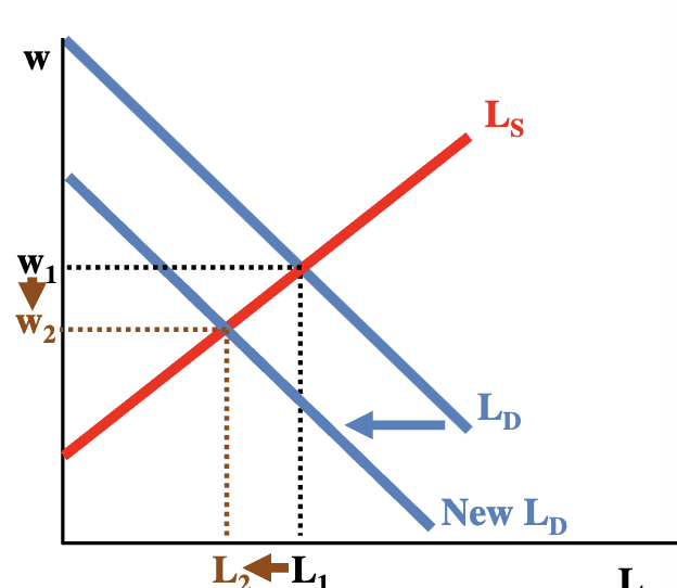
• Based on this analysis for labor markets a decrease in the demand for labor will decrease the equilibrium quantity of labor, meaning that equilibrium balances the Ls and Ld (which would mean there is no unemployment before or after this demand shift)
• This analysis presupposed competitive markets
• But it isn’t perfectly competitive.

- Many employers (buyers)

- Many workers (sellers)

- No single employer & no unions

But, remember Vernon Smith’s studies—models based on perfectly competitive markets can be predictive even without fulfilling all conditions:

• Aggregate labor demand and supply are also more

competitive than individual markets.

Y=F(A,K,eL)

• Human capital means workers aren’t homogenous—so
• labor isn’t completely interchangebale.
• • Unemployed blacksmiths might not be able to find jobs
• in the biosciences.
• • This means that there will be transition costs, including
• unemployment.
• Thus, there would be no gap between LS and LD.

• But wages are sticky—the do not adjust so easily.

• Employers typically wait for inflation to lower the value of their employees’ wages rather than directly cutting them.
• This means that we might see w* > w2, leading to LD > LS.

Labor Markets and Unemployment:

• According to the market analysis, the equilibrium wage

will adjust to balance the supply and demand for labor.

Defining Unemployment:

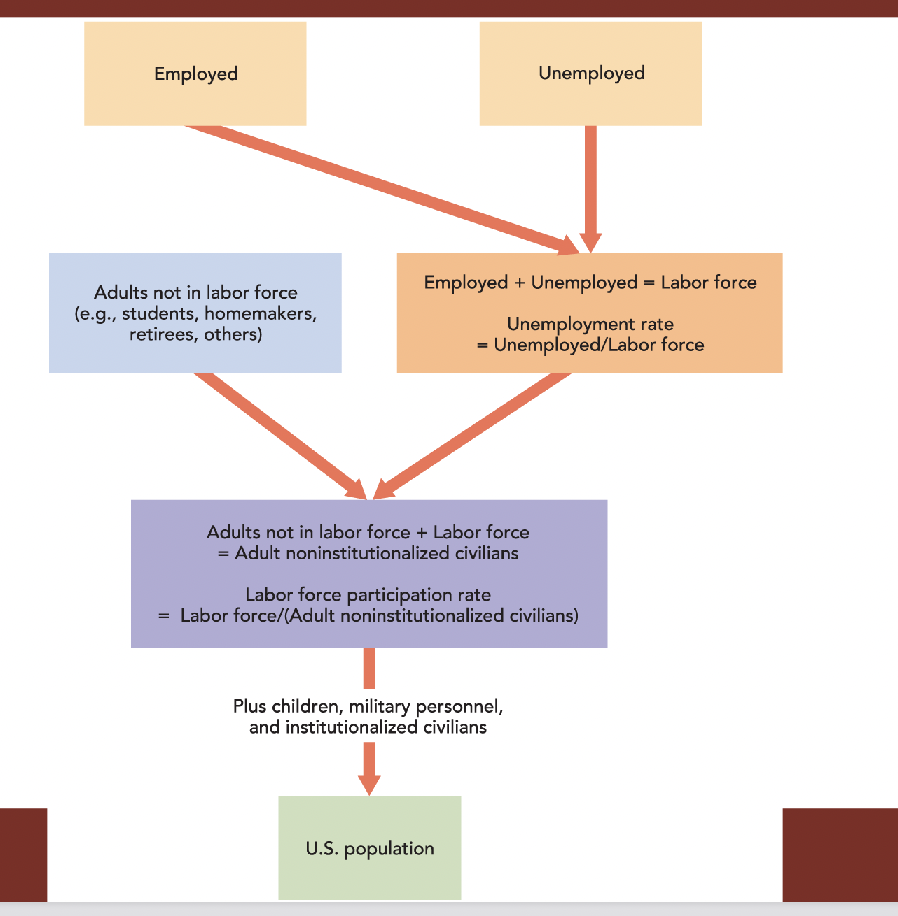
Defining Unemployment and the Labor Force:

• Those age 16+ who are not in the military or institutionalized are considered the working-age population (258 million people in 2018)
• Working-age people who are working are called employed (156 million people in 2018)
• Working age people without a job but who are looking are unemployed
• To be counted as unemployed, a person must be: 16 years or older, not instutituionalized, a civilian, and looking for work

Defining Unemployment:

• The employed as well as unemployed make up the labor force
• If neither employed nor unemployed, a person is referred to as not in the labor force
• GDP per capita was our best measure of economic prosperity
• More generally, rates will allow for easier comparisons across states, countries and time than absolute numbers
• Thus, instead of

- the total number of people in the labor force

- the total number of people unemployed

• We usually talk about

- the unemployment rate

- the labor force participation rate: Labor force/civilian noninstitutional population x 100

• Unemployment rate = unemployed/labor force = unemployed/unemployed+employed x 100

Chapter 12 Notes:

Defining and Measuring Inflation-

• Inflation is an increase in the average level of prices and is measured through an index
• Inflation is measured by changes in a price index and the inflation rate is the percentage change in a price index from one year to the next
• Inflation rate = P2-P1/P1 x 100
• P2 is the index value in year 2 and P1 is the index value in year 1. A 10% inflation rate means that goods and services are priced 10% higher than they were a year ago.
• Shifts in supply and demand push prices up and down all the time
• Inflation is an increase in the average level of prices. For example, some prices in year 1 go up and some go down, but overall the average level of prices is 100. Inflation tends to lift all prices so by year 10 the average level of prices is 200.

Price Indexes:

Economists measure inflation using several different price indexes that are based on different bundles of goods:

1. Consumer Price Index: Measures the average price for a basket of goods and services bought by a typical consumer and covers some 80,000 goods and services and is weighted so that an increase in the price of a major item like housing counts more than an increase in the price of a minor item like kitty litter.
2. GDP deflator: The ratio of nominal to real GDP multiplied by 100. It covers all finished goods and services
3. Producer Price Indexes: Measure the average price received by producers. Unlike the CPI and GDP defaltor, producer price indexes measure prices of intermediate as well as finished goods and services

• CPI is the measure of inflation that corresponds most directy to their daily economic activity
• The basket of goods and services brought by the average consumer is changing all the time. For example, the CPI, contains a category for audio media like music
• If the Bureau of Labor Statistics measured the price of music by the price of vinyl records today, it would report that there has been a tremendous increase in the price because vinyl records are now expensive collector’s items. To avoid this problem, the BLS periodically updates the basket to reflect the introduction of new goods

Inflation in the United States and Around the World:

• Since 1950 in the U.S., the average inflation rate over this period was 3.6%, but in many periods, especially in the 1970s, inflation was significantly higher. Over the past 10 years (2010-2020), inflation in the U.S. has averaged about 1.8%

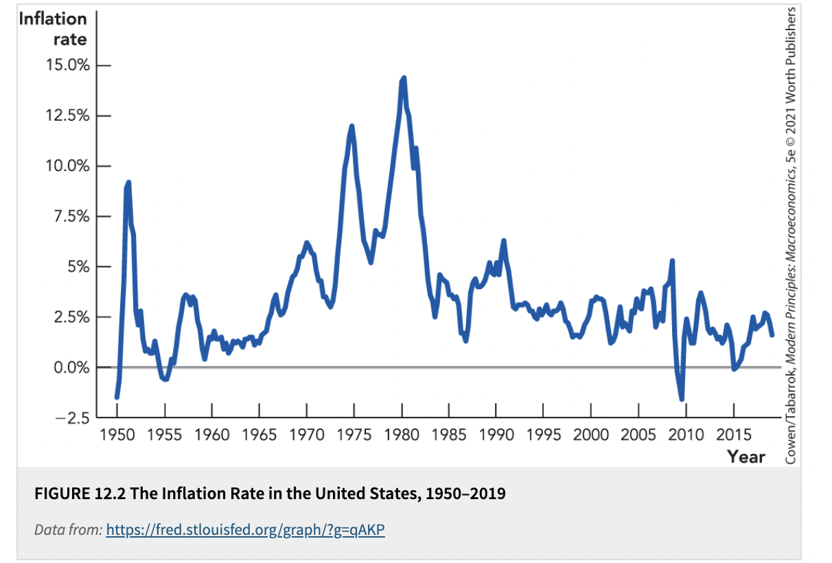
• In the U.S. a basket that cost about $10 in 1913 would have cost $36.70 in 1969, $100 in 1982, $207 in 2007, and $256 in 2019.
• Real price: A price that has been corrected for inflation; used to compare the prices of goods over time. These are used to compare the prices of goods over time. Example: The price of a gallon of gasoline was $1.25 in 1982 but double that, $2.50, in 2006. These prices are correct, but it should not be concluded that gasoline was twice as expensive in 2006 than in 1982. The CPI was 100 in 1982 and 202 in 2006, so the price of most products doubled in this time period as well. Therefore, the price of gasoline didn’t increase over this time period relative to other goods
• Recent U.S. inflation experience is moderate compared with international inflation rates and the historical record
• Hungary’s postwar hyperinflation is the largest on record. What cost 1 Hungarian pengo in 1945 cost 1.3 septillion pengos at the end of 1946.

The Quantity Theory of Money:

• The quantity theory of money sets out the general relationship between money, velocity, real output, and prices. It also helps to explain the critical role of the money supply in determining the inflation rate
• Example: You are paid $4,000 every month and you spend $4,000. In a year, you spend $4,000 12 times, so your total yearly spending is $48,000. The formula for yearly spending is this: M x v = P x Yr where M is the money you are paid, v is the number of times in a year that you spend M, P is prices, and Yr is a measure of the real goods and services that you buy. Both sides of the equation are also equal to nominal GDP.
• Over the period we are interested in, real GDP is fixed by the real factors of production: capital, labor, and technology
• In the previous scenario, v was 12 because you paid monthly. In the U.S. economy today, v is about 7 and is determined by the same kind of factors that might determine your personal v, factors such as whether workers are paid monthly or biweekly, how long it takes to clear a check, and how easy it is to find and use an ATM

The Cause of Inflation:

Mv=PYr, when v and Y are fixed, increases in M must cause increases in P

• If Yr is fixed by the real factors of production and v is stable, then it follows immediately that the only thing that can cause increases in P are increases in M, the supply of money.
• Inflation is caused by an increase in the supply of money
• The quantity theory of money can also be written in terms of growth rates. We denote the growth rate of any variable with a little arrow over the variable so M with an arrow on top is the growth rate of the money supply, P with an arrow on top is the growth rate of prices, and so forth. If Mv=PYr, then it is also true that: M (arrow on top) + v (arrow on top) = P (arrow on top) + Y(arrow on top)r
• The growth rate of prices is also known as inflation (inflation is often written with the pi symbol
• Yr (with an arrow on top), the growth rate of real GDP, is relatively low, say between 2% and at most 10%. If these two factors are ignored, M (with an arrow on top) is approximately equal to the Inflation rate (pi).
• The growth rate of the money supply will be approximately equal to the inflation rate according to the quantity theory of money
• Inflation is always and everywhere a monetary phenomenon (Nobel Prize-winner Milton Friedman)
• Even though large and sustained increases in prices stem from increases in the money supply, changes in v and Yr can have modest influences on inflation rates
• Example: If M and v are fixed, then increases in Yr (real GDP) must lower prices
• Changes in the velocity of money will affect prices. For example, increases in the velocity of money can accelerate an already existing inflation.
• At the height of the German hyperinflation in 1923, prices were increasing by the minute
• In an economic panic, individuals may simply hold their money and be afraid to spend it
• Deflation: A decrease in the average level of prices, that is, a negative inflation rate
• Disinflation: A reduction in the inflation rate
• The quantity theory assumes changed in M cannot change Yr. In the long run, this makes sense because real GDP is determined by capital, labor, and tech and changes in M won’t change any of these factors. In the long run money is neutral.
• However, it’s possible changes in M can change Yr in the short run. Under some circumstances increases in M can temporarily increase real GDP and decreases in M can temporarily decrease real GDP.

Inflation Example (fake scenario):

• Consider a mini economy consisting of a baker, tailor, and carpenter who buy and sell products among themselves
• A government consisting of a mini economy in Zimbabwe for instance starts paying its soldiers with newly printed money.
• Due to this, there is more of a demand for goods like bread or clothes
• The baker, tailor, and carpenter are making more goods, but the price of goods that they may want to purchase for themselves has gone up due to inflation from the soldiers purchasing most of all available goods
• Although they earned more dollars, their real wages (amount of goods they can buy) have decreased
• As new money enters the economy, the baker, for example, will rush to the tailor/carpenter to spend before prices rise. Unfortunately, everyone would have had the same idea, resulting in prices increasing even more quickly as the time before.
• Eventually the citizens should be able to expect and prepare for inflation
• An unexpected increase in the money supply can boost the economy in the short run, but as firms and workers come to expect and adjust to the new influx of money, output will not grow any faster than normal.

The Costs of Inflation:

• Inflatiuons tends to be more variable and thus more difficult to predict when the inflation rate is high, therefore when it occurs, it is a surprise to many.
• In the U.S., inflation was 1.3% in 1964; the rate more than quadrupled to 5.7% in 1970 and increased to 11% per year by 1974
• For example, inflation in Peru went from 77% in 1986 to 7,500% in 1990 and then back down to 73% in 1992
• Inflation destroys the ability of market prices to send signals about the value of resources and opportunities
• Prices are signals and inflation makes price signals more difficult to interpret. In our inflation parable, for example, the baker initially though that the increase in they demand for bread signaled that the real demand for bread had increased. Since all prices were rising, the real demand had technically not increased. If one day the real demand for bread does increase, only now the baker is so used to inflation, he ignores the signal. Instead of working harder, the baker continues to bake the same amount, missing opportunities because signals have become obscured
• It is difficult to sort out the relative strength of the influences for money supply increasing or real demand increasing
• Example: If the price of a movie goes up to 10% and other prices including wages go up by about the same amount, the real price of a movie has stayed more or less the same
• Money illusion: The false perception that occurs when people mistake changes in nominal prices for changes in real prices. When people mistake changes in nominal prices for changes in real prices
• Inflation usually confuses consumers, workers, firms, and entrepreneurs.
• When price signals are difficult to interpret, the market economy doesn’t work as well–resources are wasted in activities that appear profitable but in fact are not, entrepreneurs are less quick to respond to real opportunities, and resources flow more slowly to profitable uses

Inflation Redistributes Wealth:

• Inflation is a type of tax
• The inflation tax does not require tax collectors, a tax bureaucracy, or extensive record keeping
• Money-strapped governments in danger of collapsing typically use massive inflation. Almost all the hyperinflations involved governments with massive debts or spending that couldn’t be paid for with regular taxes.
• Example: A lender lends money at an interest rate of 10% but that over the course of the year the inflation rate is also 10%. The lender has earned a return of 10%-- called the “nominal return”. But the lender’s real rate of return is paid 10% interest, but she is paid in dollars that have become 10% less valuable. Thus, the lender’s real rate of return is 0%.
• Inflation can reduce the real return that lenders receive on their loans, in effect transferring wealth from lenders to borrowers.
• Example: In the 1970s, high inflation rates meant the real value of 30-year fixed-rate mortgages that were taken out in the 1960s declined tremendously, redistributing billions of dollars from lenders to borrowers (burrowers benefited but many lenders went bankrupt)
• In the late 1970s, however, many people began to expect that 10% inflation was here to stay, so home buyers were willing to take out long-term mortgages with interest rates of 15% or higher. When inflation fell unexpectedly in the early 1980s, borrowers found their payments were much higher; wealth was redistributed from borrowers to lenders.
• Real interest rate = Nominal rate - Inflation rate
• R real = i - pi
• The real rate of return is equal to the nominal rate of return minus the inflation rate
• Nominal rate of return: The rate of return that does not account for inflation
• When lenders expect inflation to increase, they will demand a higher nominal interest rate
• Example: If lenders expect that the inflation rate will be 7% and the equilibrium real rate is 5%, then lenders will ask for a nominal interest rate of approximately 12%.
• The tendency of nominal interest rates to increase with expected inflation rate is the Fisher Effect

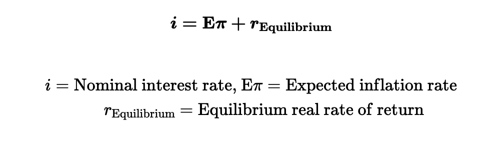
• Nominal interest rate is equal to the expected inflation rate plus the equilibrium real interest rate
• The Fisher effect says that the nominal rate will rise with expected inflation

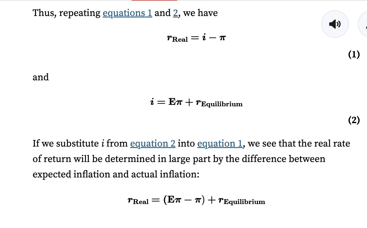
• If Epi<pi, expected inflation is less than actual inflation, then the real rate of return will be less than the equilibrium rate and will quite possibly be negative. Wealth will be redistributed from lenders to borrowers
• Only when Epi=pi is when expected inflation is equal to actual inflation, will the real return be equal to the equilibrium return
• There will be no unexpected redistribution of wealth between borrowers and lenders
• Governments are often borrowers so governments benefit from unexpected inflation
• A government with massive debts has a special incentive to increase the money supply–called monetizing the debt
• Monetizing the debt: The result of government paying off its debts by printing money
• If lenders expect the government will inflate its debt away, they’ll only lend at high nominal rates of interest, so to avoid this, the government may try to make a credible promise to keep a low inflation rate (the Fisher effect)
• The U.S. debt is increasingly owed to foreigners, which makes some economists predict a return of inflation in the U.S.

Inflation and the Breakdown of Financial Intermediation:

• When nominal interest rates aren’t allowed to rise and the inflation rate is high, the real rate of return will be negative
• When real interest rates turn negative, many take their savings out and use cash to invest abroad or to buy a real asset like land that would appreciate in value alongside inflation, or simply consume more
• When more people due this, the supply of savings declines and financial intermediation becomes less efficient

Hyperinflation and the Breakdown of Financial Intermediation:

• When inflation is volatile and unpredictable, long-term loans become riskier and they may not be signed at all. The real problem of unexpected inflation isn’t simply that it redistributes wealth, but that few long term contracts will be signed when borrowers and lenders both fear that unexpected inflation/deflation could redistribute their wealth
• Any contract involving future payments will be affected by inflation
• Unexpected inflation redistributes wealth throughout society in arbitrary ways. When the inflation rate is high and volatile, unexpected inflation is difficult to avoid and society suffers as long-term contracting grinds to a halt

Inflation Interacts with Other Taxes:

• Most tax systems define incomes, profits, and capital gains in nominal terms
• Example: You bought a share of stock for $100, and over several years inflation alone pushed its price to $150. The U.S. tax system requires you pay profits on the $50 gain even though the gain is illusory
• Inflation leads to people paying capital gain taxes when they should not
• For example, a single-filer in GA who earned $10,000 would pay $230 on their first $7,000 and 5.75% on the remaining $3,000- $230 + 0.0575 x 3000 = $402.50 (or 4.025% of their total earnings)
• Suppose the nominal rate of return is 10%, the inflation rate is 7%, and the capital gains tax is 30%. What would be the nominal and real post-tax returns?

Inflation is Painful to Stop:

• When workers, firms, and consumers expect 10% inflation, a lower rate is a shock. At first, firms may interpret the lower rate as a reduction in real demand and thus they may reduce output and employment
• Workers may be thrown out of work as the unexpected increase in their real wage makes them unaffordable

Some Takeaways:

• Inflation is an increase in the average level of prices as measured by a price index such as the consumer price index

March 13th Notes:

• Across countries, Spain has the highest employment rate at 15.3%, and most of continental Europe has a much higher rate of unemployment in the U.S., whose unemployment rate is 3.7%

Defining Unemployment:

• Unemployment can be financially/psychologically devastating
• Underemployment means the economy is underperforming

Labor Force Participation:

• (LFPR) is the percentage of the adult, noninstitutionalized, civillian population who are working or actively looking for work
• LFPR = Unemployed + Employed/Adult population = Labor force/Adult population x 100
• In September 2023 the LFPR was 168 million/264.4 million x 100 = 63.5%

Labor Force Participation and Lifecycle:

• Labor force participation is affected by lifecycle effects and changing demographics. Those ages 16-19 participate 34%, 25-24 participate 80.9%, and 65+ is 18.6%

Two Explanations for Falling Labor Force Participation:

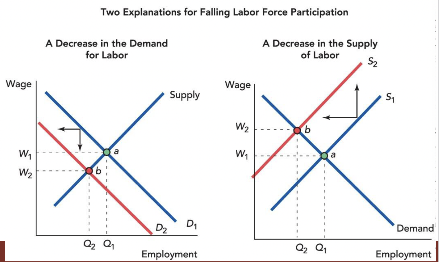
Discouraged Workers:

• Workers who have given up looking for work but who would still like a job
• Difficult to measure because the concept isn’t well defined
• One definition is workers who want and are available for work, and who would have looked for a job sometime in the last year but not in the last month because they believe no jobs were available for them
• The number of discouraged workers is small relative to the number of unemployed workers

Underemployment

• The unemployment rate also doesn’t measure the quality of the jobs or how well workers are matched to their jobs

- A taxi driver with a PhD in chemistry is counted as fully employed; so is a part-tine worker

• Defining and measuring partial employment is difficult, so the Bureau of Labor Statistics measures involuntarily part-time workers to capture the problem of underemployment

Alternative Measures of Unemployment:

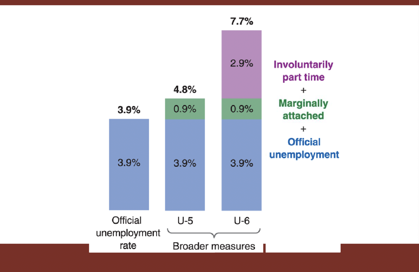
Understanding Unemployment:

• Unemployment can be broken down into three types based on their sources:

- Frictional unemployment

- Structural unemployment

- Cyclical unemployment

• Frictional and structural unemployment will combine to explain a society’s natural, long-term unemployment rate

Frictional Unemployment:

• Finding a job that you want at a wage that you will accept and that the employer will pay takes time, leading to frictional unemployment
• Frictional unemployment is short-term unemployment caused by the ordinary difficulties of matching employees to employers
• Scarcity of information is one of the causes of frictional unemployment

Duration of Unemployment:

• One of the most worrying aspects of the 2007-2009 recession was the increase in long-term unemployment

Frictional Unemployment:

• Is typically a large share of total unemployment because the U.S. economy is dynamic
• Innovation and competition drive progress, which creates new jobs and destroys old jobs: “creative destruction”
• In Feb 2014, 4.59 million new jobs were created, but there were also 4.38 million job separations, for a total of 210,000 new jobs

Structural Unemployment:

• Persistent, long-term unemployment caused by long lasting shocks or permanent features of an economy that make it more difficult for some workers to find jobs
• Structural unemployment has significant costs:

- Loss of economic output

- The unemployed suffer higher levels of stress, higher rates of suicide, and lower rates of measured happiness

Structural Unemployment Cont:

• One cause is large, economy-wide shocks like oil shocks
• It has become a more serious problem in Europe than the U.S. because of labor regulations
• Unemployment benefits, minimum wages, unions, and employment protection laws benefit workers
• All of these regulations are more generous and wide-ranging in Europe
• But the regulations can increase unemployment rates

Minimum Wages:

• The bigger the gap between the minimum wage and equilibrium wage, the more unemployment it causes
• This gap tends to be bigger in Western Europe than the U.S.

- Minimum wages especially effect young workers with limited skill

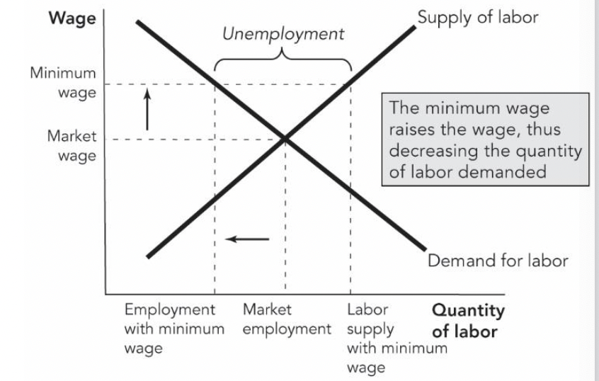
Unions:

• An association of workers that bargains collectively with employers over wages, benefits, and working conditions
• Unions can provide value for workers and employers alike
• Excessively strong unions have an effect similar to minimum wages
• Unions are more powerful in Europe than in the U.S.

Employment Laws:

• Under the employment at-will doctrine, an employee may quit, and an employer may gire an employee at any time for any reason. There are many exceptions, but it’s the most basic U.S. employment law
• Employment protection laws have the following effects:

- Create valuable insurance for workers will full-time jobs

- Make labor markets less flexible and dynamic

- Increase the duration of unemployment

- Increase unemployment rates among young, minority, or otherwise “riskier” workers

Employment Protection Laws:

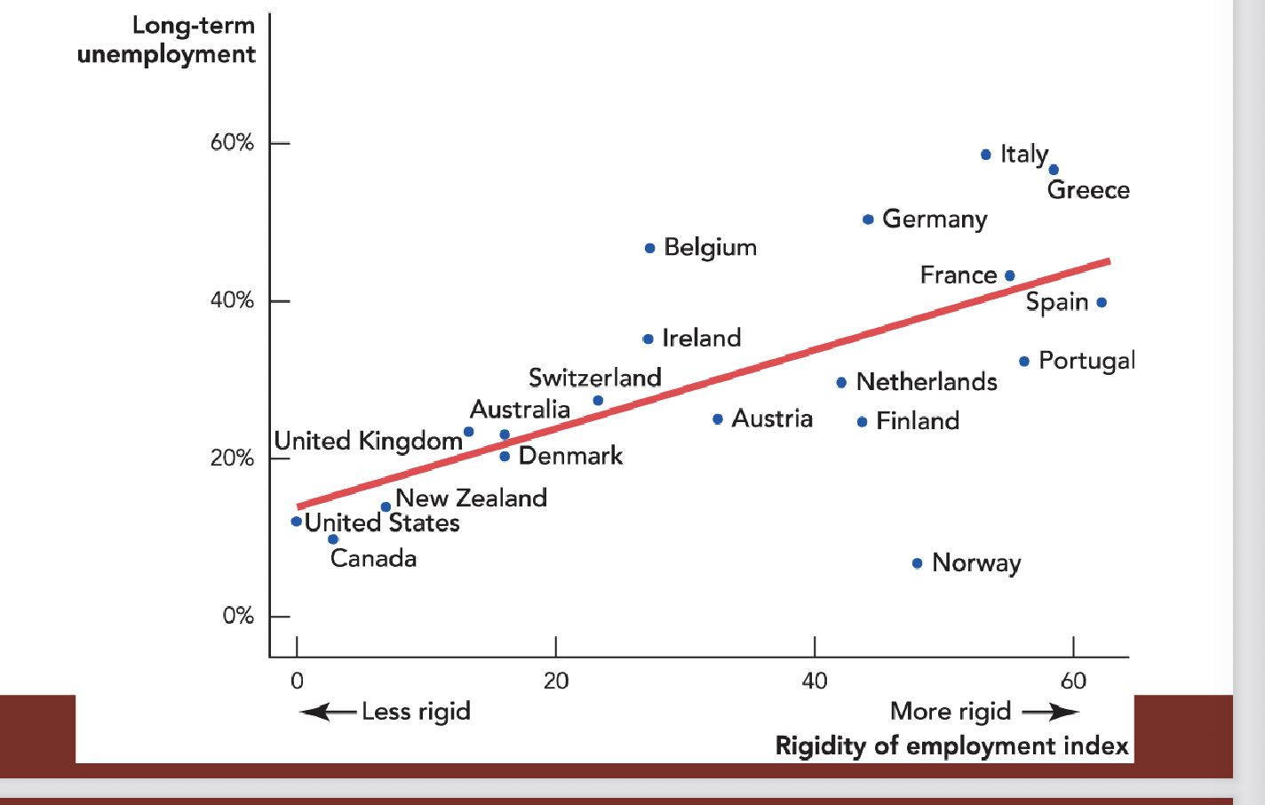
Active Labor Market Policies:

• Polices such as work tests, job search assistance, and job retraining programs that focus on getting unemployed workers back to work
• These can help reduce structural unemployment

Structural Unemloyment:

Factors that can increase structural unemployment-

• Large, long-lasting shocks that require the economy to restructure

- Oil shocks, shifts from manufacturing to services, globalization, and technology shocks

• Labor regulations

- Unemployment benefits, minimum wages, powerful unions, and employment protection laws

Factors that can reduce structural unemployment-

• Job retraining, job-search assistance, work tests, and early employment bonuses

Cyclical Unemployment:

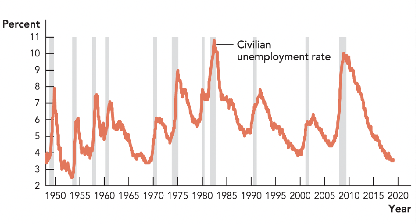
• Cyclical unemployment is unemployment correlated with the business cycle
• Unemployment increases dramatically during a recession for two reasons:

1. When GDP is falling, firms often lay off workers, which increases unemployment
2. Idle labor and idle capital hurt the economy’s ability to create more jobs

March 15th Notes:

Natural Unemployment Rate:

• Cyclical unemployment can increase or decrease dramatically over a matter of months
• When thinking about long-run employment patterns, it can thus be helpful to focus on the natural unemployment rate–that is, the sum of structural unemployment and frictional unemployment.

Chapter 12:

• Zimbabwe President Robert Mugabe’s policy of seuizing commercial farms drove away entrepreneurs and investors
• To bribe his enemies

Defining Inflation:

• Inflation is an increase in the average level of prices

- In other words, inflation is a decline in the purchasing power of money.

• Not all price increases are inflation

- Remember that demand increases or supply decreases can both raise the price of a particular good

- Inflation, however, is a general increase in prices

- These can be hard to distinguish in real time

Inflation Rates:

• Inflation is measured by changes in a price index
• To calculate inflation rate (pi) we find the percentage change in a price index from one year to the next (P2-P2/P1 x 100, where P2 is the index value in year 2 and P1 is the index value in year 1)

Example: If the price index is 200 in year 1 and 210 in year 2, the rate of inflation is 5% (210-200/200 x 100)

Price Indexes:

1. Consumer Price Index (CPI): Measures the average price for a basket of goods and services bought by a typical American consumer, covers 80,000 goods and services and is weighted so major items count more
2. GDP deflator: The ration of nominal to real GDP multiplied by 100; covers finished goods and services
3. Produce price indexes (PPI): Measure the average price received by producers; includes intermediate and finished goods and services

Consumer Price Index:

• Measures the average price for a basket of goods and services bought by a typical American consumer; covers 80,000 goods and services and is weighted so major items cost more
• For most Americans, CPI is the measure of inflation that corresponds most directly to daily economic activity
• The Bureau of Labor Statistics computes the CPI and tries to take both new goods and higher-quality goods into account when computing the CPI

Constructing CPI:

• The BLS identifies what the average household typically buys
• Each of these categories contain many different goods and services
• The BLS then collects prices from stores where people do their shopping and tallies up the price of the basket of goods and services. Inflation rates are calculated based on this price index

Example:

A dog is adopted and gets 730 cans of dog food, 6 cans of kibble, 2 vet visits, and 2 chew toys. In year 1, cans of dog food were 1.80 dollars each, kibble was 40 dollars each, vet visits were 60 dollars each, and chew toys were 10 dollars each. 1.8 x 730 = 1314 + 6 x 40 = 240 + 2 x 60 = 120 + 2 x 10 = 20 = 1694 dollars. For year 2, cans cost 1.85, kibble 41, vet visits 65, and chew toys 11. 1.85 x 73 + 41 x 6 + 65 x 2 + 11 x 2 = 1,749

1749/1694 x 100 = 103.2

Challenges with Measurement:

New Goods Bias-

• New goods that were not available in the base year appear and, if they are more expensive than the goods they replace, they put an upward bias into the CPI

Quality Change Bias-

• Quality improvements occur every year. Part of the rise in the price is payment for improved quality and is not inflation
• The CPI counts all the price rise as inflation

Commodity Substitution Bias-

• The market basket of goods used in calculating the CPI is fixed and doesn’t take into account consumers’ substitutions away from goods whose relative prices increase

Outlet Substitution Bias-

• As the structure of retailing changes, people switch to buying from cheaper sources, but the CPI, as measured, doesn’t take into account of this outlet substitution.

Example:

3025-2650/2650 x 100 = 14%

March 18th Notes:

• Money is any asset regularly used in transactions
• Money in the U.S. consists of

- currency

- deposits at banks and other depository institutions

• Money in th eUnited States today is fiat money, because it has no intrinsic value
• Before fiat money, people used:

- Barter – people exchange goods for goods

- Commodity money–money that has intrinsic value such as gold or silver coins

Functions of Money:

Medium of exchange → Money is used to buy goods and services

Unit of account → Money is a common unit used to measure economic value

Store of value → Money can be saved

Medium of Exchange-

• A medium of exchange is an object that is generally accepted in exchange for goods and services
• In the absence of money, people would need to exchange goods and services directly, which is called barter
• Barter requires a double coincidence of wants, which is rare, so barter is costly

Unit of Account-

• A unit of account is an agreed measure for stating the prices of goods and services
• Money simplifies comparisons
• Easier to apply opportunity cost principle

Functions of Money-

Store of value-

• Money can be held for a time and later exchanged for goods and services

Defining Inflation:

• Inflation is an increase in the average level of prices

- In other words, inflation is a decline in the purchasing power of money

• Not all price increases are inflation

- Remember that demand increases or supply decreases can both raise the price of a particular good

- Inflation, however, is a general increase in prices

Inflation Rates:

• Inflation rates (pi) are measured by changes in a price index from one year to the next

GDP Deflator formula: pi=p2-p1/p1 x 100 Where P2 is the index value in year 2 and P1 is the index value in year 1.

• We call a decrease in the average level of prices (a negative inflation rate) deflation
• We call a reduction in the inflation rate–even when prices are still rising–disinflation

Price Indexes:

1. Consumer Price Index (CPI): Measures the average price for a basket of goods and services bought by a typical American consumer; covers 80,000 goods and services and is weighted so major items count more
2. GDP Deflator: The ratio of nominal to real GDP multiplied by 100; covers finished goods and services
3. Producer Price Indexes: Measure the average price received by producers; includes intermediate and finished goods and services

Consumer Price Index:

• Measures the average price for a basket of goods and services bought by a typical American consumer; covers 80,000 goods and services and is weighted so major items count more
• For Americans, CPI is the measure of inflation that corresponds most directly to their daily economic activity
• CPI=cost of cpi basket of current prices/cost of cpi basket at base-period prices x 100

Challenges with Measurement:

• The CPI’s fixed consumption basket can lead it to overstate the true inflation rate due to:

- New goods bias

- Quality change bias

- Commodity subtitution and outlet substitution biases

• The BLS now tries to take both new goods and higher-quality goods into account when computing the CPI, but some of this bias still remains

New Goods Bias:

• New goods that were not available in the base year appear and, if they’re more expensive than the goods they replace, they put an upward bias into the CPI

Quality Change Bias:

• Quality improvements occur every year. Part of the rise in the price is payment for improved quality and is not inflation
• The CPI counts all the price rise as inflation

Commodity Substitution Bias:

• The market basket of goods used in calculating the CPI is fixed and doesn’t take into account consumers’ substitutions away from goods whose relative prices increase

Outlet Substitution Bias:

• A structure changes, people switch to cheaper sources

The Magnitude of the Bias:

• An estimate made in 1996 says that the CPI overstates inflation by 1.1 percentage points a year
• The BLS has now corrected much of the bias, but some still may remain

GDP Deflator:

• Price index that tracks the price of all goods and services produced domestically and the ratio of nominal GDP to real GDP
• Nominal gdp/rela gdp x 100
• Tells how much the overall price level differs from the real GDP’s base year
• If the GDP deflator with a 2017 base was 109.76 in 2021 and 117.02 in 2022, we can calculate the inflation rate: 117.02-109.76/109.76 x 100 = 6.6%

GDP Deflator vs CPI:

• Prices of capital goods

- Included in GDP deflator (if produced domesticlaly)

- Excluded from CPI

• Prices of imported consumer goods

- Included in CPI

- Excluded from GDP deflator

• The basket of goods

- CPI: fixed

- GDP deflator: changes every year

Producer Price Index:

• Measures the average selling prices received by domestic producers for their output

- The BLS calculates the PPI using a method much like it uses to produce the CPI but based on a different “basket” of goods

- Unlike CPI or the GDP deflators, the basket for PPI includes both intermediate and finished goods and services

What Inflation Do We Use For…:

• The CPI is the most widely accepted measure of the change in cost of living
• Automatically adjusting wages, benefits, tax brackets, and the like to compensate for inflation is called indexation
• Monetary policy focuses on the personal consumption expenditure deflator
• The federal reserve sets its inflation target using th epersonal consumption expenditure (PCE) deflator

- Like CPI, it focuses on household consumption

- Unlike CPI, PCE’s basket is not fixed so there’s no substitution bias: PCE deflator = nominal PCE/ real PCE x 100

• Forecasters look for the underlying trends in inflation

- Prices on food and energy markets can be volatile for reasons that involve the forces of S+D on these specific markets

- This can limit their value when forecasting inflation

• Forecasters use core inflation, which excludes food and energy (Core CPI or Core PCE)

Alternate Measures of Inflation:

• Different measures of inflation are better suited for different tasks

- The CPI is used for cost-of-living adjustments

- The PCE deflator is used by the Federal Reserve

- Core inflation is used by forecasters

- The producer price index and the GDP deflator are used by businesses

Real Prices:

• Prices that have been corrected for inflation and used to compare the prices of goods over time
• Real price = nominal pricet x Po/Pt, where Po is the value of the price index in the base year and Pt is the value of the price index in the year the nominal price being adjusted came from
• Typically, we will use the CPI to calculate real prices

Real Prices Examples:

1. Comparing how 1955’s prices for McDonalds compares with today’s prices, set Pt as the CPI for 1955 and Po as the CPI for 2023 for milkshakes:

Real price = 20 cents x 304.4/26.8 = 2.27 dollars

A medium vanilla shake now is $4.49

Definitions

• The money supply (M) is the total volume of money held by the public at a particular point in time

- This not only includes physical cash in circulation but also deposits in commercial banks

- Can also include other relatively liquid assets, depending on inclusive a measure of supply is (M1 v. M2 v. M3)

• The velocity of money (v) is the average number of times a dollar is spent on finished goods and services in a year

- V refers to how fast money passes from one holder to the next

Quantity Theory of Money:

• The quantity theory of money sets out the general relationship between money, velocity, real output, and prices
• Mv=PYr (both sides of this equation are equal to nominal GDP)
• PYr is the price level times real GDP
• Mv is the total amount spent on finished goods and services (money supply)
• V is the velocity of money
• P is the price level
• Yr is the real GDP
• Real GDP is fixed by the real factors of production
• The velocity of money is determined by factors that change only slowly, such as how often workers are paid, or how long it takes to clear a check

- In the U.S., the velocity of money is about 7.

• We assume that both real GDP (Yr) and velocity (v) are stable compared to the money supply (M).
• If Yr is fixed by the real factors of production and v is stable then the only thing that can cause an increase in P is an increase in M
• The quantity theory of money implies inflation is caused by increases in the supply of money.

- It says that the growth rate of the money supply will app. equal the inflation rate

Monetary Growth and Inflation:

“Inflation is always and everywhere a monetary

phenomenon.”

—Milton Friedman (1912–2006

The Cause of Inflation:

• An increase in the supply of money will only cause inflation in the long run
• An unexpected increase in the money supply can boost the economy in the short run
• As firms and workers come to expect and adjust to the new influx of money, output will not grow any faster than normal
• Thus, money is neutral in the long run

The Costs of Inflation:

Four problems associated with inflation-

1. There is price confusion and money illusion
2. Inflation redistributes wealth
3. Inflation interacts with other taxes
4. Inflation is painful to stop

Price Confusion and Money Illusion:

• Inflation makes price signals more difficult to interpret
• It’s not always clear whether prices are rising due to increased demand or rising due to an increase in the money supply
• Sometimes we mistake inflation for higher wages and prices in real terms
• When people mistake changes in nominal prices for changes in real prices, they fall prey to the money illusion
• Money-illusion leads to short-run tradeoff between unemployment and inflation
• In 1958 A.W. Phillips identified this relationship
• Economic policymakers increasingly tried to take advantage of this tradeoff

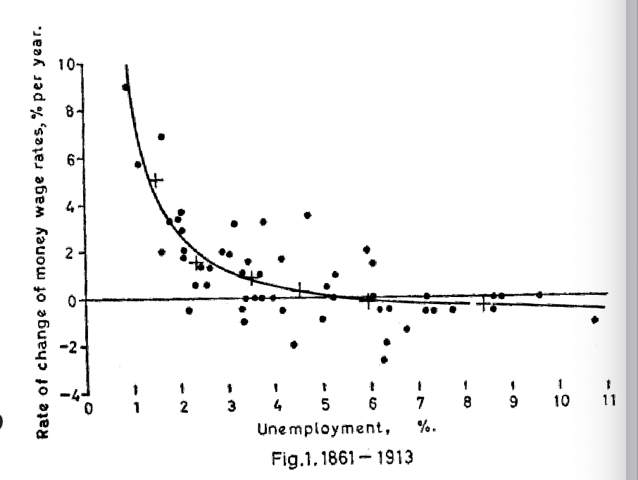
Price Confusion and Money Illusion:

• When people are fooled by money illusion, resources are wasted in activities that appear profitable but aren’t and resources flow more slowly to profitable uses
• Eventually, people start to expect inflation–so they stop getting fooled by the money illusion
• Thus, the economy faces inflation and stagnation, or “stagflation”

Inflation Redistributes Wealth:

• Inflation acts like a type of tax that transfers real resources from citizens to the government
• Unexpected changes in inflation rates also transfer wealth between lenders and borrowers by changing the real return on loans

- A lender’s nominal rate of return is his/her rate of return without accounting for inflation

- A lender’s real rate of return is his/her nominal rate of return minus the inflation rate

• A lender’s real rate of return is equal to the nominal rate of return minus the inflatiuuon rate

- R real = i - pi where

- R real = Real interest rate

- i = Nominal rate of interest

- Pi = Rate of inflation

• Thus, higher levels of inflation mean lenders need a higher nominal interest rate to realize the same real rate of return

The Fisher Effect:

• With higher levels of inflation, lenders need a higher nominal interest rate to realize the same real rate of return
• If lenders expect inflation to increase, they’ll demand a higher nominal interest rate

- This tendency for nominal interest rates to rise with expected inflation rates is called the Fisher Effect

• Says that the nominal interest rate is equal to the expected inflation rate plus the equilibrium real interest rate

i=Epi+Requilibrium where

Requilibrium = Equilibrium real rate of return

i=Nominal rate of interest

Epi=Expected rate of inflation

• Nominal interest rates tend to increase with inflation rates

Inflation Redistributes Wealth:

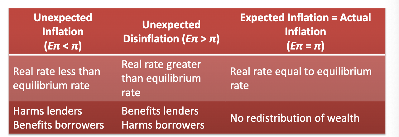
• When governments monetize debt (pay off their debts by printing money), it effectively acts as a tax on everyone
• A government with massive debts has an incentive to increase the money supply since it benefits from unexpected inflation
• The government doesn’t always inflate its debt away for two reasons:

- If lenders expect inflation, they’lll increase nominal rates

- Buyers of bonds are often also voters, who would be upset of real returns were shrunk

March 22nd Notes:

Introduction:

• Business fluctuations are fluctuations in the growth rate of real GDP around its trend growth rate
• A recession is a significant, widespread decline in real income and employment
• To understand booms and recessions, you can develop a model of aggregate demand

Suppose the nominal rate of return is 8%, inflation rate is 5%, and capital gains tax is 25%

(1-t) x i = (1.25)(8)

Inflation Interacts with Other Taxes:

• If asset prices rise due to inflation, people pay capital gains taxes when they should not
• We need to adjust earnings to reflect the real rate of return

- An asset’s real rate of return is equal to the nominal rate of return minus the inflation rate (r=i-pi)

• But governments typically tax nominal returns

- People effectively pay taxes on the inflation rate as well as their real earnings

Example:

• Suppose the nominal rate of return is 12% the inflation rate is 10% and the capital gains tax is 25%
• To calculate the nominal return after tax, you would deduct the tax from the nominal return

(1-t) x i = (1-.25) x 12% = 9%

• To calculate the real return after tax, we would deduct the inflation rate from the nominal after-tax return since the tax would apply to the full nominal value:

r after tax = i after tax - pi = 9% - 10% = -1%

• Suppose the nominal rate of return is 10%, the inflation rate is 7%, and the capital gains tax is 30%.
• What would be the nominal and real post-tax returns?
• To calculate our nominal return after tax, we would deduct the tax from the nominal return:
• (1-t) x i = (1-.3) x 10% = 7%
• To calculate our real return after tax, we would deduct the inflation rate from the nominal after-tax return since the tax would apply to the full nominal value
• R after tax = i after tax - pi = 7% - 7% = 0%

Aggregate Demand Curve:

• Shows all combinations of inflation and real growth that are consistent with a specified rate of spending growth M + v
• The AD curve can be derived using the quantity theory of money in dynamic form M + c = P + Yr where

M = Growth rate of the money supply

V = Growth in velocity

p=Growth rate of prices

Yr=Growth rate of real GDP

The equation can also be written as: M + v = Inflation + Real growth

• Example:

- If money growth = 5%, velocity growth = 0%, and real growth is 0%, the inflation rate = 5%.

- If money growth = 5%, velocity growth = 0%, and real growth is 3%, the inflation rate = 2%

The Aggregate Demand Curve:

• An AD curve with a slope of -1 means a 1 percentage point increase in real growth reduces inflation by 1%.

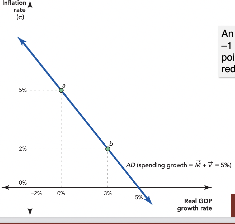
M + v = Inflation + real growth

Shifts in Aggregate Demand Curve:

• Increased spending must flow into either a higher inflation rate or a higher growth rate

- If spending growth increases, because of either an increase in money supply or an increase in velocity, then the AD curve shifts up and to the right

• A decrease in spending growth shifts the AD curve f

1. Increases in spending growth, increase in M and/or increase in v shift the AD curve to the right
2. Decreases in spending shifts the AD curve to the left

Chapter 13 Notes:

• Real GDP in the U.S. has grown at an average rate of 3.2% per year over the past 65 years.
• The economy advances and recedes, rises and falls, and booms and busts
• The growth rate might drop to -5% in a typical recession, and sometimes the economy can grow at a rate of 7-8% or higher
• Business fluctuations: Fluctuations of real GDP around its long-term trend or “normal” growth rate
• Recessions: Significant, widespread declines in real income and employment.
• Recessions are of special concern to policymakers because unemployment increases during a recession
• A recession is a time when all kinds of resources, not just labor but also capital and land, are not fully employed.
• To understand booms and recessions, a model of aggregate demand and aggregate supply (AD-AS) is used. The AD-As model has three curves: the aggregate demand curve, long-run aggregate supply curve, and the short-run aggregate supply curve

Aggreggate Demand Curve:

• The aggregate demand curve tells us all the combinations of inflation and real growth that are consistent with a specified rate of spending growth
• Quantity theory in dynamic form can be written as: M + v = P + Yr
• M is the growth rate of the money supply, v is growth in velocity (how quickly money is turning over), P is the growth rate of prices, and Yr is the growth rate of real GDP, which can be called real growth
• M + v = Inflation + Real growth
• Example: M=5, v=0, real growth = 0, therefore 5+0=inflation + 0, so inflation = 5%.
• If money supply is growing by 5% a year, and velocity is stable at 0%, then spending is growing by 5% a year. Spending plus the same goods = higher prices
• An AD curve tells all the combination of inflation and rea growth that are consistent with a specified rate of spending growth.
• Inflation is caused when more money chases the same goods. If more money is chasing an increased quantity of goods, then all else being equal, the inflation rate will be less than the increase in money growth
• There are two comibations of inflation and real growth that are consistent with a spending growth of 5%. Point a shows an inflation rate of 2% and a real growth rate of 3%. Both of these are consistent with a spending growth of 5% and belong on the same AD curve. The AD curve is a straight line with a slope of -1, meaning that, given the rate of spending growth, a 1 percentage point increase in real growth reduces inflation by 1 percentage point.

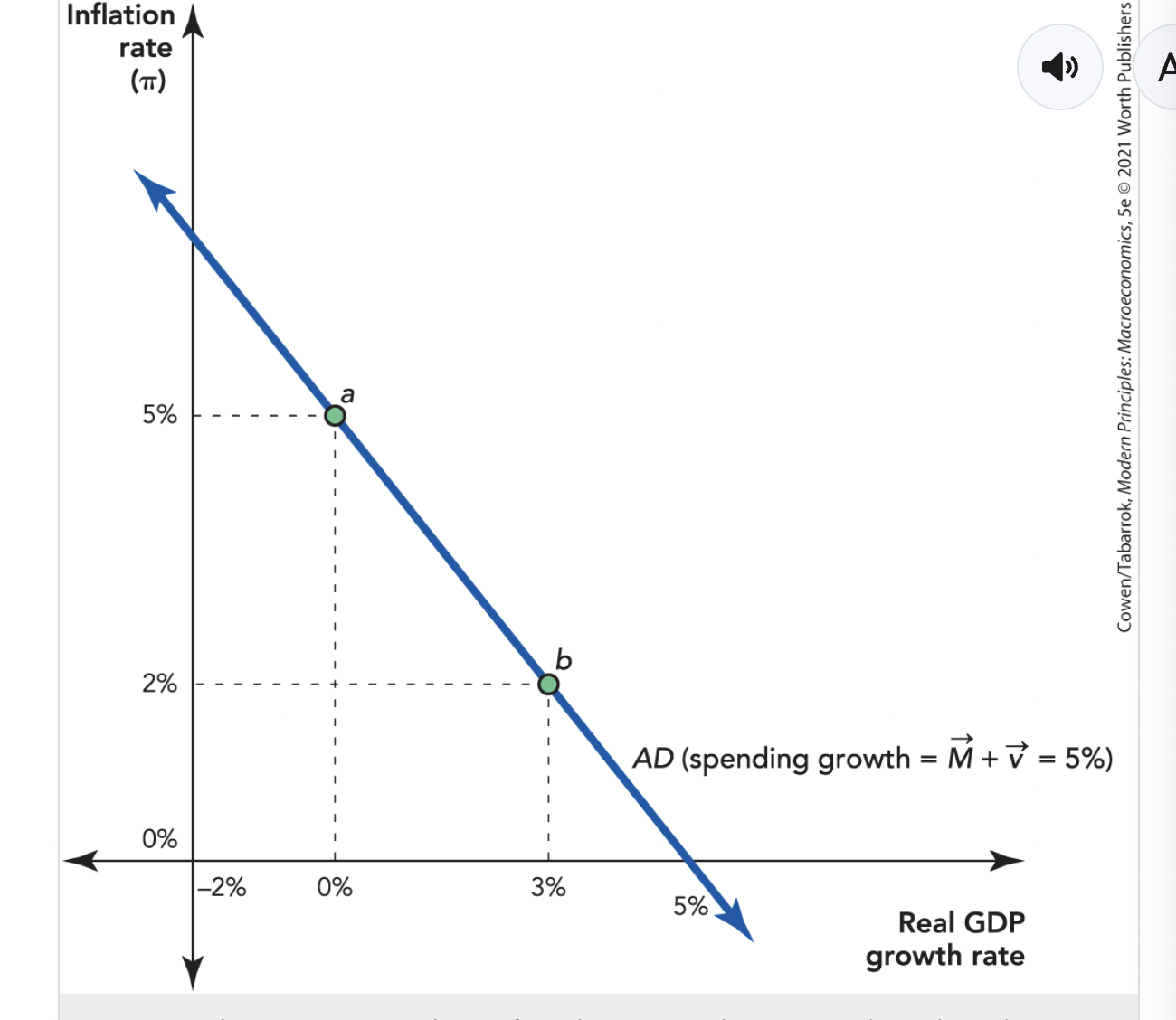
Shifts in the Aggregate Demand Curve:

• The AD curve for a spending growth of 5% is all the combinations of inflation and real growth that add up to 5%.
• All combinations of inflation and real growth along the AD curve add up to 5% and all the combinations of inflation and real growth along the AD curve denoted AD (M + v = 7%) add up to 7%.
• Increased spending must flow into either a higher inflation rate or a higher growth rate
• An increase in spending growth shifts the AD curve outward, up and to the right, and a decrease in spending growth shifts the AD curve inward

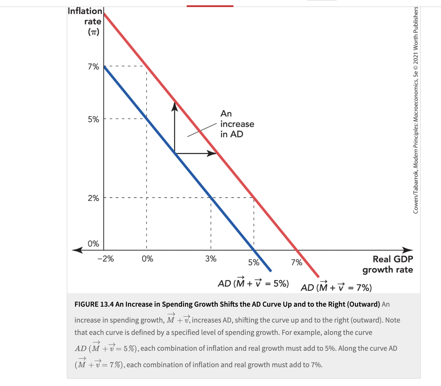
• An increase in spending growth can be caused by either an increase in M or v
• Increased spending growth shifts the AD curve outward and decreased spending growth shifts the AD curve inward

The Long-Run Aggregate Supply Curve:

• Economic growth depends on increases in the stocks of labor and capital and on increases in productivity
• Every economy has a potential growth rate given by these fundamental, or real, factors of production
• The rate of growth, as given by the real factors of production, is the “Solow” growth rate
• Solow created an important model of an economy’s fundamental growth rate
• Solow Growth rate: An economy’s potential growth rate, the rate of economic growth that would occur given flexible prices and existing real factors of production
• The long-run aggregate supply curve is a vertical line at the Solow growth rate.
• The fundamental growth rate of the economy depends on factors such as the amount of quality of labor and capital, not on the rate of inflation

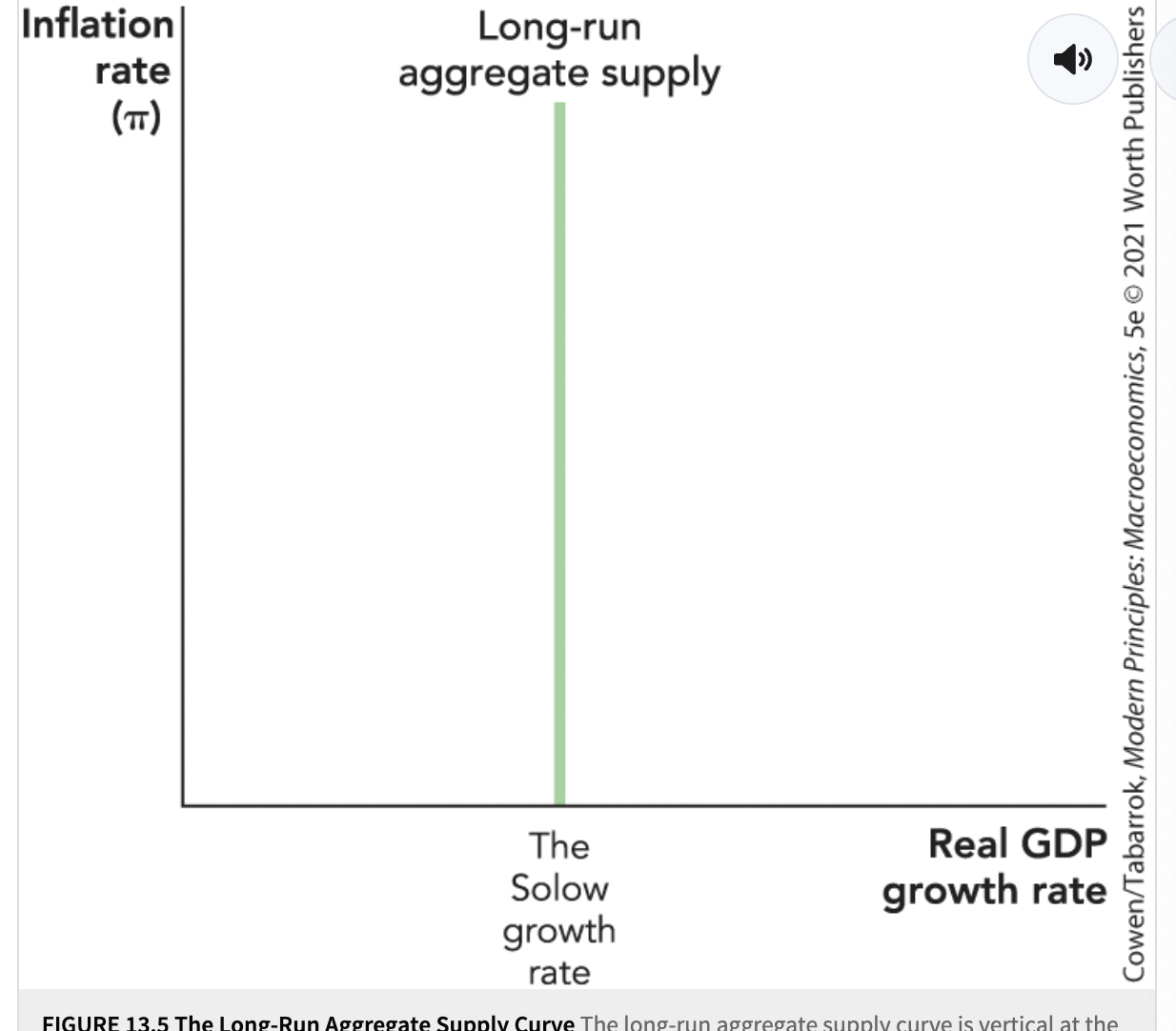
Shifts in the Long-Run Aggregate Suply Curve:

• In this model, an AD curve is shown in which the growth rate of spending is 10% a year and a long-run aggregate supply curve that has a growth ate of 3%. M + v = 10% and real growth = 3%. Inflation is 7% a year. The equilibrium inflation rate and growth rate are determined by the intersection of the AD and LRAS curves.

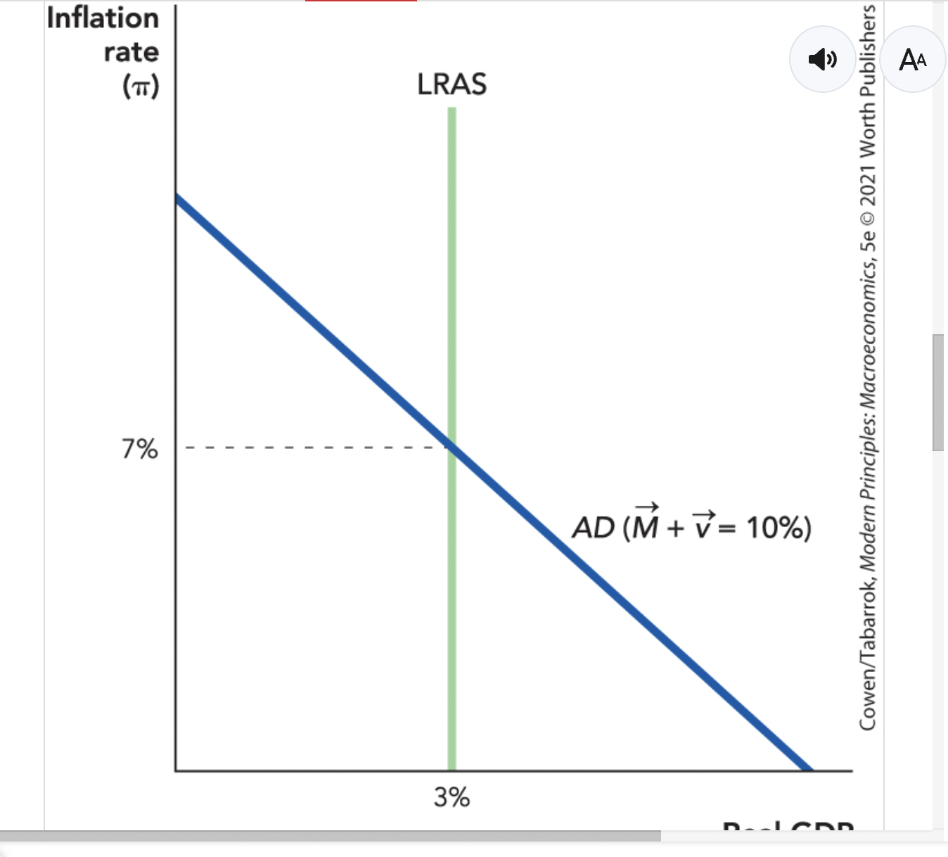
• Although the growth rate has averaged about 3% per quarter for many years, it has fluctuated around this average
• One reason growth rate fluctuates is that economies are continually being hit by shocks, which would shift the Solow growth rate. For example, consider an agricultural economy. Good weather can increase crop production while bad weather can decrease production, driving down the growth rate.
• Real shocks (aka productivity shocks) increase or decrease an economy’s fundamental ability to produce goods and services and, thus, they increase or decrease the Solow growth rate
• A positive real shock shifts the LRAS curve to the right, increasing real growth
• An increase in the supply of goods brought about by a higher real growth reduces the inflation rate
• A negative real shock shifts the LRAS curve to the left, decreasing real growth. The slower growth rate means fewer new goods to spend money on so the inflation rate increases
• For example in the 1970s a negative real shock due to the decrease in the supply of oil led to several big jumps in the price of oil.
• Shocks to the LRAS curve will change the growth rate and the inflation rate temporarily because the LRAS curve is always shifting back and forth as new shocks hit the economy
• The real business cycle is a natural extension of the Solow growth model. Business fluctuations are simply changes in economic growth in the short run driven by real shocks

Real Shocks:

• Rapid changes in economic conditions that increase or diminish the level or productivity of capital and labor, which in turn influences GDP and employment
• Agriculture has been the largest contributor to India’s GDP, so the shocks to agricultural output caused by the weather have had a big impact on GDP growth. If farmers struggle, many other sectors of the Indian economy suffer as well
• GDP boomed in 1975, growing by nearly 10%, and busted in 1979 with a decline of 5.2%
• Agriculture contributed 40% of India’s GDP in 1970, but because the Indian economy has grown and diversified it, it contributed only 20% of India’s GDP in 1990.
• In the U.S., agriculture contributes less than 1% of GDP, so yearly variations in the weather don’t have much of an effect on GDP.

Oil Shocks:

• Oils and machines are complementary, which means they work together, along with labor, to produce output
• Higher gas prices reduced the demand for larger cars and increased the demand for smaller cars
• The oil shock meant that many auto plans producing larger cars shut down or were used at less than full capacity
• Since oil is an important input in many sectors of the economy, high oil prices-or oil shocks-hurt many American industries
• Unexpected shocks are the most costly to deal with.
• Careful statistical analysis can disentangle the effect of oil shocks from the many other shocks that keep on hitting the economy
• A 10% increasein the high price of oil lowers the GDP growth rate, from what it would’ve been without the price increase, for a little more than two years
• Other possible shocks are wars, terrorist attacks, major new regulations, tax rate changes, mass strikes, and new technologies such as the Internet

Aggregate Demand Shocks and the Short-Run Aggregate Supply Curve:

• An aggregate demand shock is a rapid and unexpected shift in the aggregate demand curve
• Since the AD curve is all about spending, we can also say that an aggregate demand shock is a rapid and unexpected shift in spending
• A positive shock to spending increases output at first, but in the long run only increases prices. M + v = Inflation + real growth and an increase in spending M+v must either increase the inflation rate pi or the real growth rate
• In the long run, the real growth rate will be equal to the Solow rate, which isn’t influenced by the inflation rate, so in the long run an increase in spending will increase the inflation rate alone

Short-Run Aggregate Supply Curve:

• This is an upward-sloping curve, meaning that in the short run an increase in aggregate demand will increase both the inflation rate and the growth rate, and a decrease in demand will decrease both the inflation rate and the growth rate
• Example: The initial equilibrium is at point a, where the real growth rate is at the Solow rate (3%) and the inflation rate is 2%, and the expected inflation rate is 2%

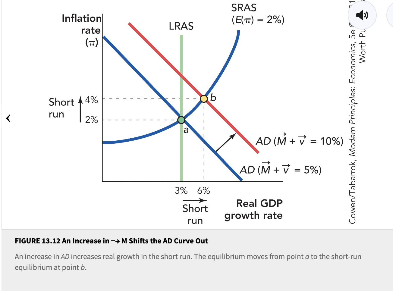
• The growth rate of the money supply increases unexpectedly from 5-10%. The injection of more money into the economy increases AD, which in turn, creates a temporary boom at point b
• Example:An increase in spending encourages the baker to expand, so she offers her workers more overtime opportunities at a higher wage. At first the workers are pleased since they see that their nominal wage–the number on their paychecks–has increased. But as the workers spend their money, they discover that prices elsewhere in the economy are rising so much that even with overtime, their wages can buy fewer goods and services. Their real wages have decreased even though their nominal wages have increased. The workers’ eagerness to work harder is a nominal wage confusion
• Economists call the costs of changing prices meny costs because the costs of printing new menus when a restaurant changes prices. Prices don’t move instantly to their new long-run equilibrium because it is costly to change prices.
• Over time, firms will begin to realize that the price of eggs, for example isn’t coming back down–the increase in price really was permanent and so firms will adjust their menus
• As prices rise and workers begin to realize that their real wage hasn’t risen, they’ll demand higher wages
• As expectations and prices adjust, more and more of they increase in M is reflected in the inflation rate and less is reflected in the real growth rate
• An increase in M increases real growth in the short run–during the period in which prices and wages are sticky
• In the long run, people will always come to expect the actual inflation rate and the economy must be on the LRAS curve intersects the new AD curve
• From an initial equilibrium at point a, the fall in AD shifts the economy to a new short-run equilibrium at point b, creating a small reduction in the inflation rate and a large reduction in real growth
• It takes time for a decrease in spending to make its way through the economy for all the reasons that we have already discussed in the case of an increase in spending-namely wages are sticky, menu costs and uncertainty make businesses reluctant to change prices immediately, and expectations take time to adjust
• In the short run, a fall in spending growth is split between a fall in inflation rates and a fall in growth
• The economist Truman Bewley interviewed employers and labor leaders, asking them why wages don’t fall during a recession
• A decrease in spending that requires expected wage growth to decrease will tend to create a large decrease in the growth rate

Shocks to the Components of Aggregate Demand:

• Changes in velocity can be thought of as increasing or decreasing the spending rate, holding the money supply constant
• National spending identity: Y = C + I + G + NX
• If v increases, the growth rate of C,I,G, or NX must increase

A Shock to C:

• C may decrease due to consumer expectations becoming more pessimistic and fearful about the economy, as they did in 2008 when the banking system was in danger of collapse
• In the short run, the economy moves from point a to point b, where the inflation rate is lower and the real growth rate is also lower–in this example at point b, growth is negative and the economy is in a recession
• In the long run, fear recedes, wages adjust, and the spending growth rate returns to normal so the economy returns to long-run equilibrium at point a

Why Changes in v Tend to be Temporary:

• M can be permanently set at any rate–5%,17%,103%--but changes in v tend to be temporary
• If nothing else changes, consumption will return to its normal growth rate
• A decrease in C reduces AD and the rate of inflation in this period
• In future periods, however, C will return to its normal rate, and as it does, AD and inflation will return to their previous rates
• Long-run or sustained inflation requires ongoing increases in the money supply
• Fear and confidence play a similar role in investment spending as in consumption spending
• When prices fall, consumers suddenly realize that their wealth has fallen so they now need to save more; thus they cut back on their spending
• Taxes are another important shifter of C and I. An increase in taxes can reduce consumption growth and a decrease in taxes can increase consumption growth
• Big increases in the growth rate of government spending will increase AD, and decreases in the growth rate of government spending will reduce AD

Aggregate Demand Shocks and the Great Depression:

• The Great Depression occured in the United States as follows. In 1929, the stock market crashed, creating a mood of pessimism among the American public.
• The fall in stock prices was a wealth shock that made many people feel poorer and so they limited their spending, causing C to fall
• In 1930, depositors lost confidence, withdrawing their money, leading to bank failures. These failures diminished aggregate demand
• The fear and uncertainty created by bank failures, rising unemployment rates, falling consumer confidence, and inconsistent policymaking in Washington also reduced investment spending
• The fear and uncertainty created by bank failures, rising unemployment rates, falling consumer confidence, and inconsistent policymaking in Washington also reduced investment spending
• In 1931, instead of increasing M, the Federal Reserve allows the money supply to contract even further.
• Bad decision making caused an additional monetary contraction during 1937-1938, which led to yet another wave of economic distress
• The decrease in aggregate demand caused prices to fall, and in turn raised the real value of debts
• While the real income of creditor banks goes up for the same reason that the real value of the debt goes up, these banks don’t have such a high propensity to spend or invest as do the deperate debtors, and so the transfer of wealth from debtors to creditors still means that aggregate demand goes down
• The Great Depression was due primarily to the great fall in aggregate demand

Real Shocks and the Great Depression:

• Bank failures are a real shock and play a key roke in bridging the gap between savers and investors, and as banks failed, this bridge collapsed
• Many small businesses relied on loans from local banks that understood these businesses, and thus many small firms were especially harmed by bank failures
• A fall in M reduced aggregate demand, which led to bank failures, which led to a reduction in the productivity of financial intermediation, a real shock
• The shock to AD creates a real shock, and in other cases, a real shock creates a shock to AD; for instance, the fear and uncertainty created by a real shock can reduce AD by inducing people to cut back on spending and investment
• Under NIRA, businesses were encouraged not to invest in machinery, and they were encouraged to raise prices by creating cartels. Under the AAA, the government paid farmers to kill millions of pigs and plow under cotton fields to increase prices. None of these facilitated much economic growth
• Most famously, the Smoot-Hawley Tariff of 1930 raised tariffs on tens of thousands of imported goods
• Retaliations against the Smoot-Hawley Tariff by other countries created a spiraling decline in world trade. When other countries raised their tariffs, U.S. exports fell
• A second negative effect of the tariff occurred because a tariff is also a negative productivity shock
• Another way of seeing this point is to recognize that a tariff has exactly the same effects as an increase in transportation costs
• The U.S. was beset during the early years of the Great Depression by a natural shock, namely the onset of the so-called Dust Bowl.
• A severe drought and decades of ecologically unstainable farming practices turned millions of acres of farmland to dust, and thousands were forced to leave their homes
• The real shocks of the Great Depression could have been absorbed without major difficulty, but in a bad year, the shocks compounded one another and made a desperate situation even worse

Conclusions:

• Real shocks: Analyzed through shifts in the LRAS curve
• Aggregate demand shocks are analyzed using shifts in the AD curve
• When you combine the aggregate demand curve, long-run aggregate supply curve, and short-run aggregate supply curve into a single diagram, you can analyze a wide variety of economic scenarios and how they affect the growth rate of the economy
• The aggregate demand curve can be broken down into changes in M and v, and slopes downward
• Changes in v can be broken down into changes in C, I, G, or NX

Chapter 14 Notes:

Intertemporal Substitution-

• When weather fluctuates, so does output and therefore so does GDP, especially in agricultural economies like India. Rainfall shocks are directly correlated with the growth rate of agricultural output and GDP
• When rainfall is below average, the same capital and labor inputs produce less agricultural output–that is the direct effect of the negative rainfall shock
• For example, when crops are bountiful, it makes sense for farmers to work from down till dusk because each hour of additional work pays a lot. But when the crops are poor, the returns to an additional hour of work are low and so farmers may rationally decide to work less. The same is true for applications of capital
• This effect is called intertemporal substitution, which means that a person or business is most likely to work hard when working hard brings the greatest return. This is substituting effort across time, and thus the expression intertemporal substitution
• When jobs are plentiful and wages are increasing, there’s a tendency for fewer people to enter college, but when jobs are scarce and wages are stagnant, more people decide to invest in an education. Students understand that the opportunity cost of getting an education falls when jobs are scarce
• The supply of labor increases in a boom and falls during a recession
• Intertemporal substitution magnifies negative economic shocks
• Intertemporal substitution can feed an economic boom and make it more intense as well. If things are going well, many people will be inclined to work harder, which will in turn increase output and make things go even better

Labor Adjustment Costs:

• Once a negative shock hits the economy, labor must adjust. Workers must look for new jobs, move to new areas, and sometimes change their wage expectations
• Labor adjustment costs are the costs of shifting workers from declining sectors of the economy to growing sectors.
• Labor adjustments to shocks aren’t always rational in the narrowly economic sense of the term. For example, if an automobile worker is laid off from the General Motors assembly line and loses their formerly unionized job, they may not be able to find the same wage elsewhere. It may take a while for that person, if thrown out of work, to admit that they must settle for a lower wage. In the meantime, they are looking for a job and may even reject offers that are as good as they will ever find
• The high cost of reversing job decisions can lead to unemployment, just as the cost of reversing investment can cause investors to wait
• The choice to move jobs involves a costly-to-reverse decision. For example, unemployed workers may need to move states to get a new job
• Changes to the world require people to adjust their jobs and their careers

Time Bunching and Network Effects:

• People often bunch their activities at common points in time. For example, most people work from 9 am to 5 pm rather than from 10 pm to 6 am
• Many economic activities bunch or cluster in time because it pays to coordinate your economic actions with those of others
• People want to be investing, producing, and selling at the same time that others are investing, producing, or selling at the same time that others are investing, producing, or selling. Economic activity tends to cluster together in time just as it clusters together in space
• The “seasonal business cycle” is one form of economic clustering. The fourth quarter of the year (October through December) brings more economic activity than any other time
• After Christmas is over, however, GDP in the next period is typically lower, but tends to grow slowly during the summer months
• Seasonal cycles help us understand some features of regular business cycles
• Once some economic activity is moving in the upward or downward direction, other parts of economic activity tend to follow that momentum in order to gain the advantages of time bunching
• Example: A negative economic shock arrives and the economy slows down in the current period. Many are less keen to work, so they save up their working for some point in the future, inducing others to cut back on their work as well.
• The time bunching effect is magnified when production is organized in networks or supply chains
• Supply chains and network effects become especially important when there are large shocks to supply or demand because a single failure along the supply chain can disrupt entire industries

Collateral Damage:

• When banks lend to firms, they typically will insist that the firm have some cash on hand, strong assets, and positive net worth (assets > debts)
• Banks are more concerned about downside risk than upside gain because if the firm does poorly, the bank could lose the entire value of its loan, but if the firm does incredibly well, the bank simply gets its loan back plus interest
• Banks don’t make a lot of investmnents in startups or firms with debts that exceed assets
• A firm’s net worth acts like a collateral for a bank–a cusion or guarantee that even if the firm fails, the firm will still have cash to pay back the loan (firm=business).
• Collateral shock: A reduction in the value of collateral; collateral shocks make borrowing and lending more difficult
• During a boom, asset prices are increasing and firms have cash flow. As a result, banks are willing to approve more loans, which makes the boom even bigger
• As an economy enters the downward phase of business cycles, asset prices fall, cash flow is reduced, and firms have lower net worth. Lenders see loans as being riskier and they cut off or restrict credit, driving more firms under, increasing joblessness and making the bust worse
• Collateral shocks also affect consumers. For example, if someone buys a house in a real estate bubble, putting no money down, and borrowing it all, once the real estate bubble burst and home prices fall, that same house decreases in value greatly, making them “underwater,” with negative equity in their house. Around 2010, nearly 20% of American homes were underwater to some degree. If that person decides to sell their house, they have to pay the full amount they bought the house with to the bank, even if they sold the house for less, which would be extremely hard to do without defaulting on their mortgage. Defaulting on a mortgage would give a negative financial value to that person
• It is common that when banks have to foreclose, the bank loses 25% or even more of that value of the home. In 2010 in the wake of the recession, about 1 in 12 houses with mortgages below $1 million were in foreclosure, meaning a lot of wealth was being dissipated
• When the nominal owner of a property doesn’t have much equity in the property, they often don’t do a good job taking care of it
• Equity: The value of the asset minus the debt
• When a bank makes too many bad loans to too many insolvent home owners, the bank itself gets a low capital value, or sometimes it is said that the bank is thinly capitalized
• When the bank itself is “underwater” the bank managers don’t do a very good job of taking care of the bank, and won’t invest in their relationship with the bank or customers. Managers fail to build up new business opportunities and will take dubious risks, not worrying about the downside. Bank employees take the same attitude because there is little value to protect and the chance of bankruptcy is fairly high.
• Banks that are going “underwater” are commonly referred to as “zombie banks,” and during 2009-2010 the number of bank failures reached an all-time high
• When asset prices fall, there is a lot of collateral damage

Conclusion:

• At least five factors amplify shocks and help bring about business downturns: labor supply and intertemporal substitution, uncertainty and irreversible investment, labor adjustment costs, the desire to bunch or cluster economic activity together, and collateral shocks
• A medium-sized negative economic shock is capable of causing a disproportionately large downturn in economic production and employment

March 25th-Chapter 13 Continued Notes:

The Aggregate Demand Curve:

• We can derive the AD curve using the quantity theory of money in dynamic form:

M + v = P + Yr = inflation + real growth where

M = growth rate of the money supply

V = Growth in velocity

P = Growth rate of prices

Yr = Growth rate of real GDP

Shifts in Aggregate Demand Curve:

Long-Run Aggregate Supply Curve:

• An economy’s long-run potential growth rate is given by these real factors of production (y=f(A,K,eL)), is called the Solow growth rate
• The long-run aggregate supply cuirve is thus a vertical line at the Solow growth rate, independent of the inflation rate
• M + V = P + Yr

AD and LRAS:

• When we put the AD and LRAS curves together, we can see how business fluctuations are caused by real shocks
• The equilibrium inflation rate and the growth rate are determined by the intersection of the AD and LRAS curves

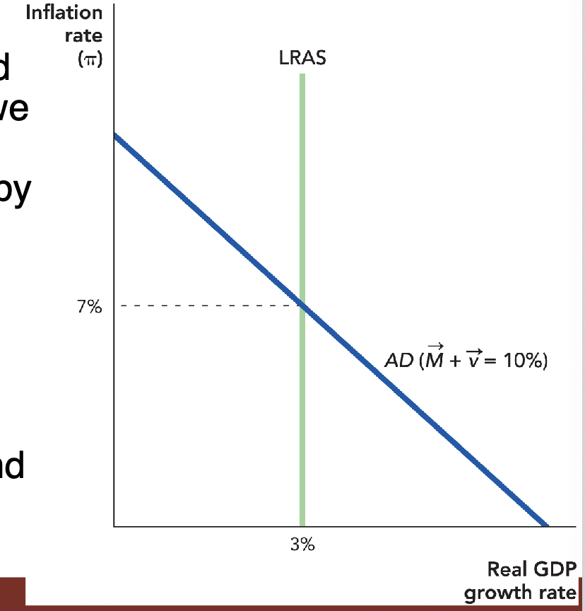
Shifts in the LRAS Curve:

• Economies are continually hit by real shocks, which shifts the Solow growth rate
• Real shocks are rapid changes in economic conditions that increase or diminish the productivity of capital and labor
• This, in turn, influences GDP and employment
• Possible shocks include wars, weather, major new regulations, tax rate changes, mass strikes, terrorist attacks, and new technologies

AD and LRAS Curves:

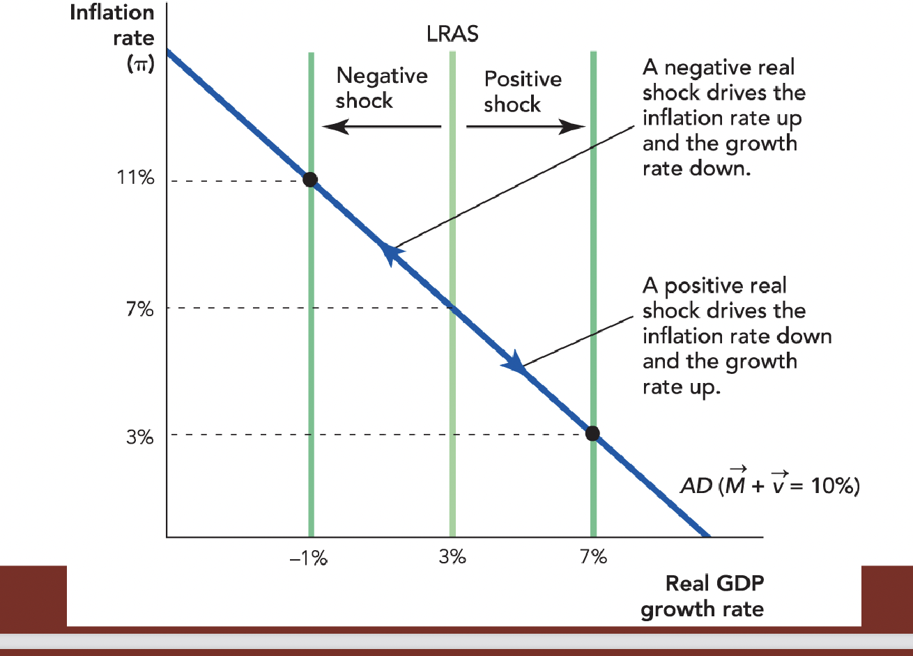
Real Shocks (Examples):

• Agriculture has been the largest contributor to India’s GDP
• If farmers struggle, many other sectors suffer
• Weather shocks influence both agricultural output and GDP
• As the Indian economy has grown and diversified, shocks due to the weather become less economically important
• Weather- Less rainfall tends to lead to less output

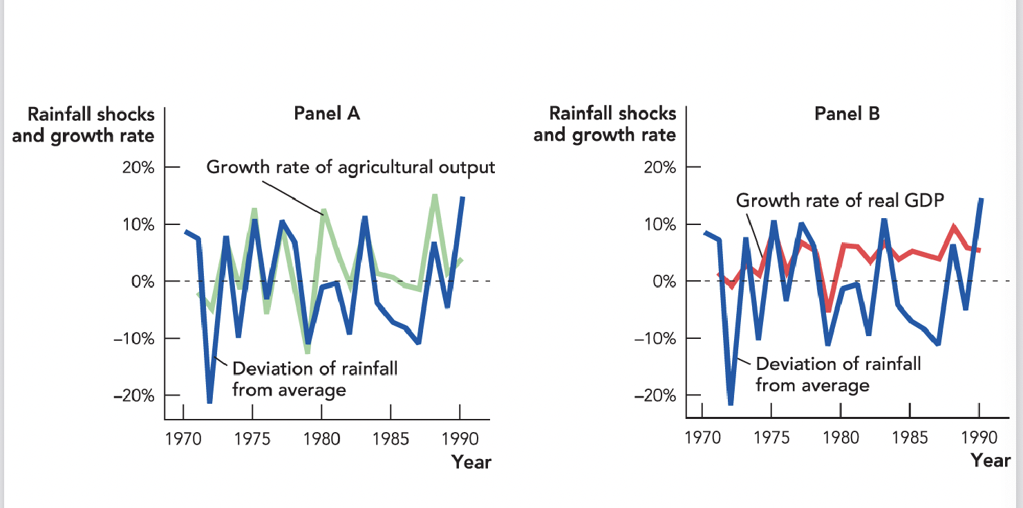
Oil-

• In an economy with a large manufacturing sector, a reduction in the oil supply reduced GDP
• Oil and machines are complementary: They work together with labor to produce output
• When the oil supply is reduced, capital and labor become less productive
• The first OPEC oil shock came in late 1973, and the price of oil more than tripled in two years
• Since oil is an important input in many sectors, high oil prices–or oil shocks–hurt many American industries
• In each of the last six U.S. recessions, there was a large increase in the price of oil just prior to or coincident with the onset of recession
• A 10% increase in the price of oil lowers the GDP growth ate for a little more than two years

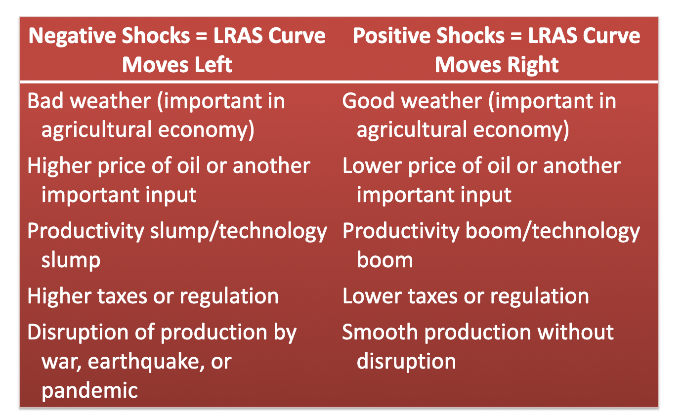
• Higher business taxes will shift the long-run aggregate supply curve to the left because higher taxes will decrease the LRAS curve.

OPEC charply reduces the quantity of oil it released to the market. The AD-AS model implies that this will lead to:

Higher inflation and lower growth

Aggregate Demand Shocks:

• John Meynard Keynes: Explained that when prices are not perfectly flexible, deficiencies in aggregate demand can generate recessions

Short-Run Aggregate Supply:

• The Short-run aggregate supply curve shows the positive relationship between the inflation rate and real growth during the period when prices and wages are sticky
• The SRAS curve is upward sloping
• In the short run, an increase in AD will increase both inflation and the growth rate
• In the short run, a decrease in AD will decrease both the inflation rate and the growth rate
• Each SRAS curve is associated with a particular rate of expected inflation E(pi)

Aggregate Demand Shocks:

• An aggregate demand shock is a rapid and unexpected shift in the AD curve (total spending growth)

- As total spending growth = M + v, aggregate demand shocks can come from either unexpected changes in the rate of money growth or the growth in the velocity of money

- These shocks can be positive or negative

• A positive shock to spending must increase either inflation or the real growth rate
• In the short run, an increase in spending will be split between increases in inflation and increases in real growth
• In the long run, the real growth rate is equal to the Solow rate, which isn’t influenced by inflation
• In the long run, therefore, an increase in spending will increase only the inflation rate

An Increase in Aggregate Demand:

• If there is an unexpected increase in M, both inflation and the growth rate increase in the short run (a—>b)

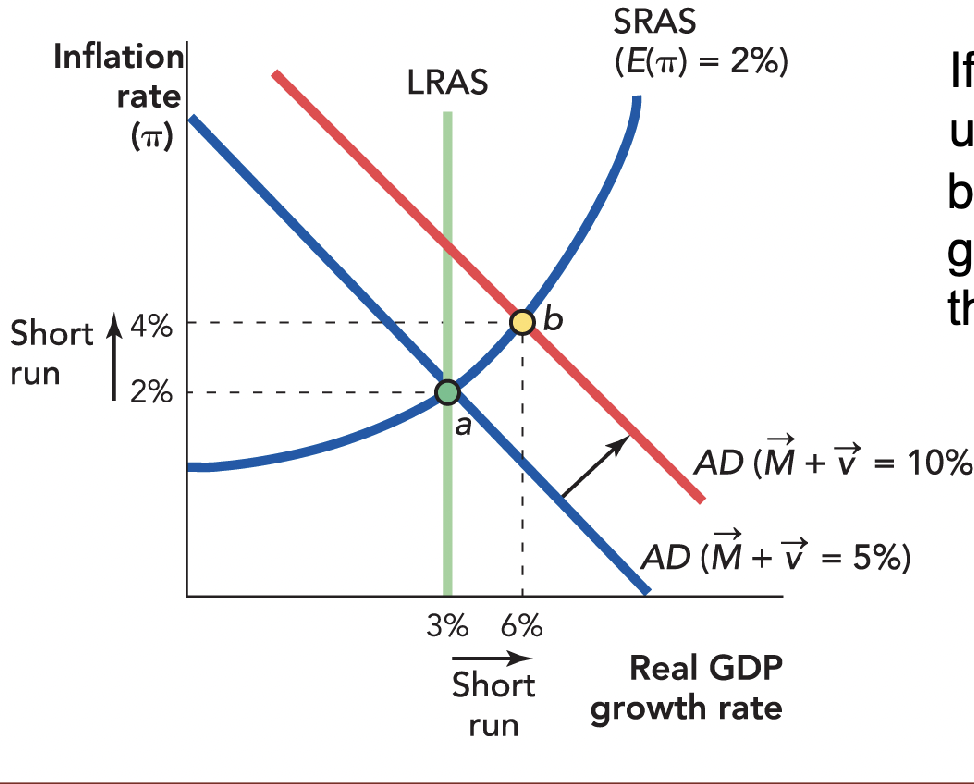
• Increases in aggregate demand bring higher nominal prices, including wages
• Workers initially mistake a nominal wage increase for a real wage increase
• The nominal wage confusion occurs when workers respond to their nominal wage instead of to their real wage–when workers respond to the wage number on their paychecks rather than to what their wage can buy in goods and services (the wage after correcting for inflation)
• Prices don’t move instantly, because it is costly to change prices (“menu costs”)

- Menu costs are the costs of changing prices

• Firms may also hold off on making price changes because they aren’t sure

whether the change in market conditions is temporary or permanent

- As prices increase throughout the economy, workers demand even higher wages to catch up to the higher inflation rate

- Eventually, inflation expectations adjust, wages become unstuck, and the growth rate returns to the Solow rate (b→c)

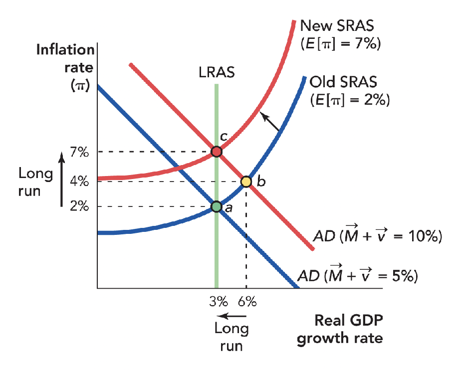
A Decrease in Aggregate Demand:

• When aggregate demand (AD) falls due to a fall in the money supply:

- The economy shifts to a new short-run equilibrium point

- The inflation rate is reduced

- Real growth is reduced (recession)

• Prices and wages are especially sticky in the downward direction
• It can take the economy a long time to move out of a recession
• A decrease in AD can induce a lengthy recession

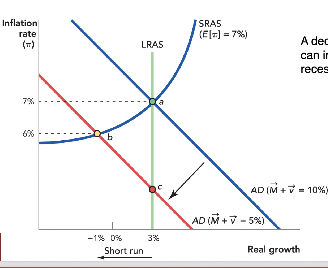
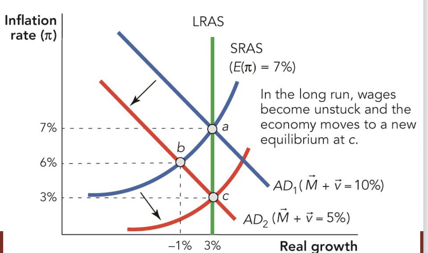
Shocks to Components of AD:

Changes in v:

• Are the same as changes in the spending rate, holding M constant
• Can be broken down into changes in the growth rate of C,I,G, or NX
• Changes in v tend to be temporary
• The shares of GDP devoted to C,I,G, and NX have been quite stable over time
• A shock to v will look different in the long run because it tends to be different

March 27th Notes:

Aggregate Demand Shocks:

• Keynes saw aggregate demand as a large source of recessions

Short-Run Aggregate Supply:

• Shows the positive relationship between the inflation rate and real growth during the period when prices and wages are sticky

Decrease in Aggregate Demand:

• If there is an unexpected decrease in M people will misinterpret the drop in total spending as a drop in demand for real goods (the money illusion). Given sticky wages and menu costs, this will decrease the
• In the long run, wages become unstuck and the growth rate returns to the Solow rate (b→c)
• When aggregate demand falls due to a fall in the money supply:

- The economy shifts to a new short-run equilibrium point

- The inflation rate is reduced

- Real growth is reduced (recession)

• Prices and wages are especially sticky in the downward direction
• A decrease in AD can induce a lengthy recession
• It can take the economy a long time to move out of a recession

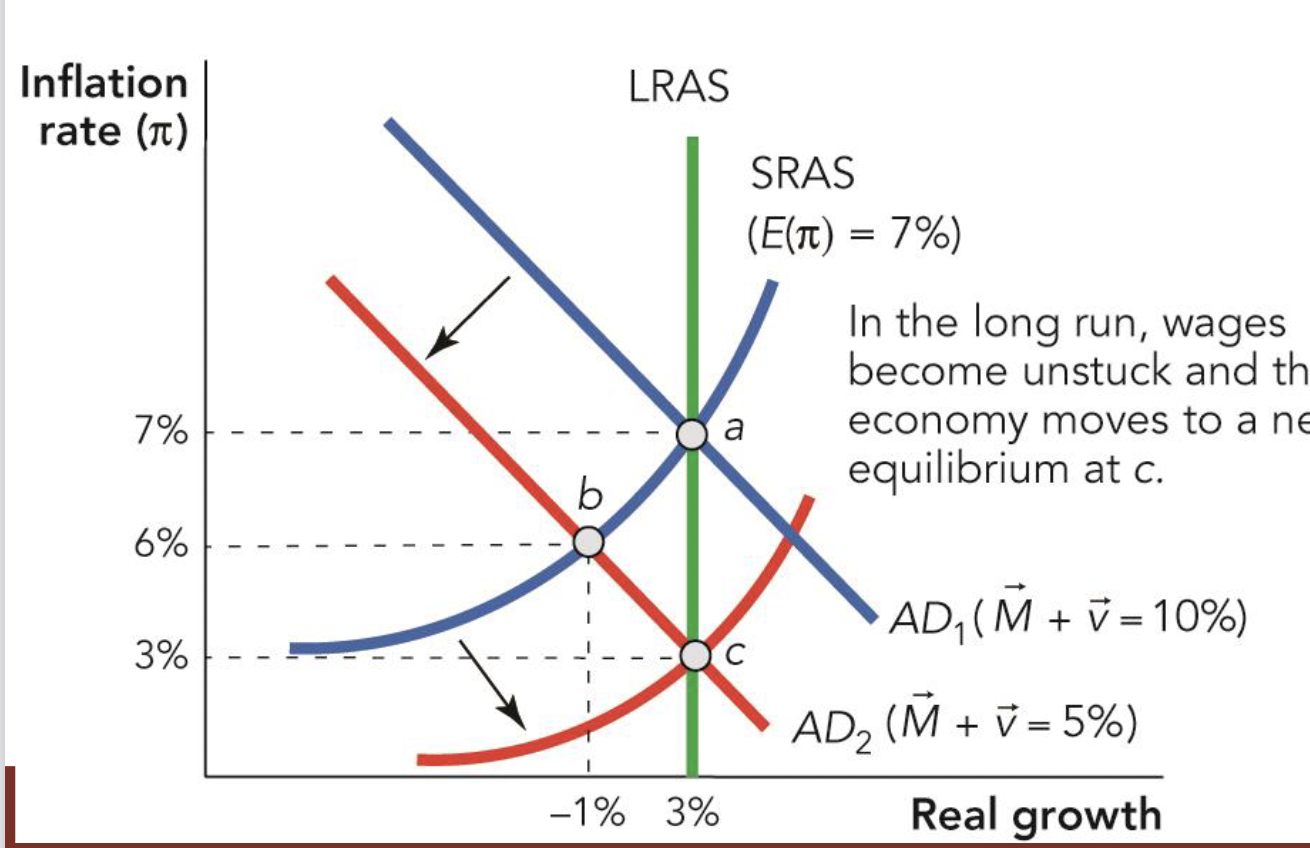
A Shock to the Growth Rate of Spending:

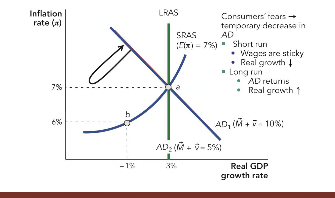
Factors That Shift AD:

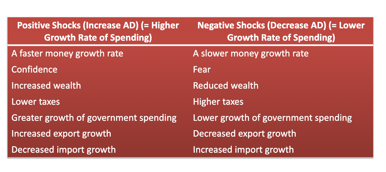
• In the long run when the economy experiences a negative shock to the growth rate of investment, points on the sras curve will converge back to its original points

The Great Depression:

• Amid the resulting recession, depositors lost confidence in their banks
• From 1930 to 1932, there were four waves of banking panics, during which >40% of America’s banks failed
• Many people lost their life savings
• Spending decreased, which meant that many businesses lost their customers and revenue
• Fear and uncertainty also reduced investment spending
• The U.S. capital stock was lower in 1940 than it had been in 1930
• In 1931, instead of increasing the money supply to boost the economy, the Federal Reserve allowed the money supply to contract even further
• Additional monetary contraction occurred from 1937 to 1938, prolonging the Great Depression
• During the early 1930s, the U.S. money supply fell by about one-third, the largest negative shock to aggregate demand in American history

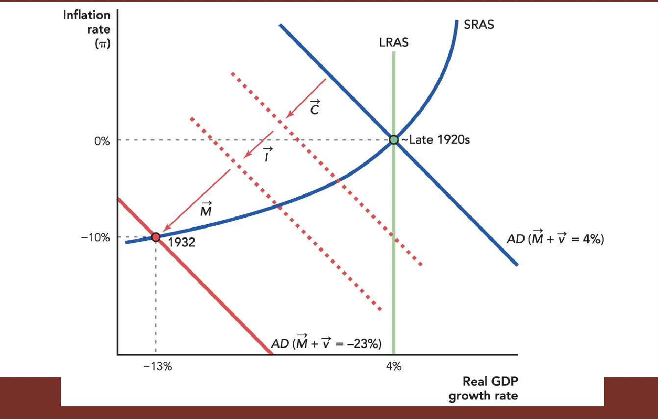
• Real shocks also played a role in the Great Depression
• Bank failures not only reduced the money supply and spending (AD shock), but also reduced the efficiency of financial intermediation
• Economic policy mistakes also impeded recovery; government agencies tried to increase prices by reducing supply
• The Smoot-Hawley Tariff of 1930 raised tariffs on imports; other countries retaliated
• A severe drought and decades of ecologically unsustainable farming practices turned millions of acres of farmland into a “dust bowl”
• The shocks compounded one another and made a desperate situation even worse
• The aggregate demand and supply model can be used to analyze fluctuations in the growth rate of real GDP
• Real shocks are analyzed through shifts in the LRAS curve, while aggregate demand shocks are analyzed using shifts in the AD curve
• Nominal wage and price confusion, sticky wages and prices, meny costs, and uncertainty create an upward-sloping short-run aggregate supply curve
• The Great Depression resulted from an unfortunate, concentrated, and interrelated series of aggregate demand and real shocks
• It can be illustrated using the AD–AS model

Chapter 14-Lecture Notes:

• Economic forces can amplify shocks and transmit them across sectors and through time
• A mild negative shock can be transformed into a serious reduction in output
• A positive shock can be transformed into a serious reduction in output
• Real shocks and aggregate demand shocks can interact, with one leading to the other

There are five transmission mechanisms:

1. Intertemporal substitution
2. Uncertainty and irreversible investments
3. Labor adjustment costs
4. Time bunching and networth effects
5. Collateral damage

Intertemporal Substitution:

• People are most likely to work hard when hard work brings the greatest return
• People’s substituting their consumption, work, and leisure across time to maximize well-being is called intertemporal substitution
• When there is a downturn people work less as well as invest less
• The ripple effects turn an initial shock into a broader recession
• Intertemporal substitution can also feed an economic boom and make it more intense

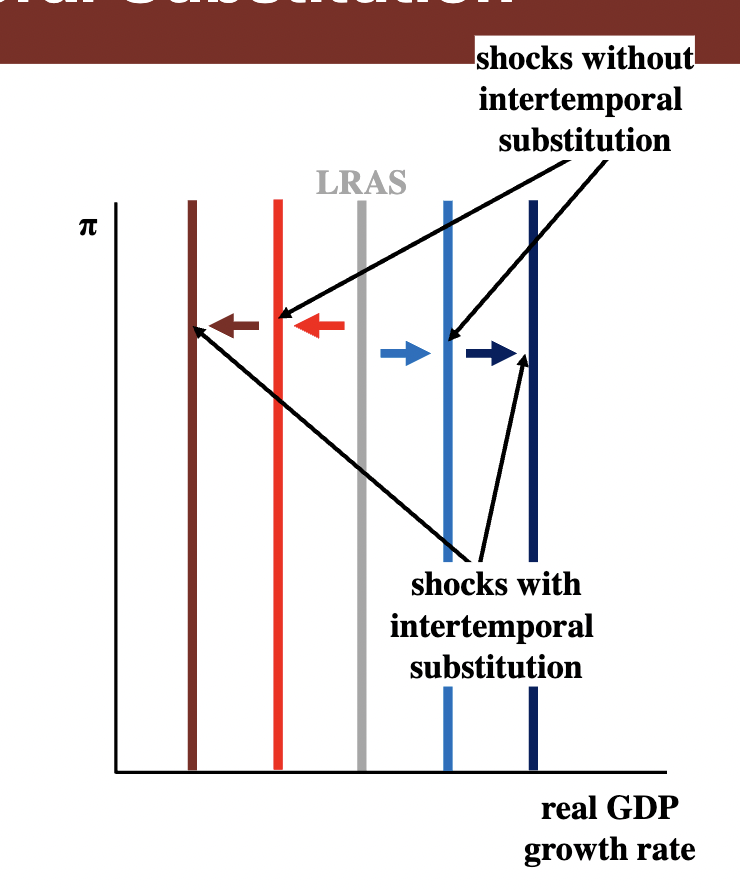
Irreversible Investments:

• Many investments involve sunk costs–they are irreversible investments, or very costly to reverse

- Irreversible investments have high value only under specific conditions–they can’t be easily moved, adjusted, or reversed if conditions change

• Once a building is built, it’s difficult to redeploy the materials to different economic uses
• The more uncertain the world appears, the harder it is for investors to read signals about where they should invest
• Uncertainty usually slows investment and keeps resources in less productive uses

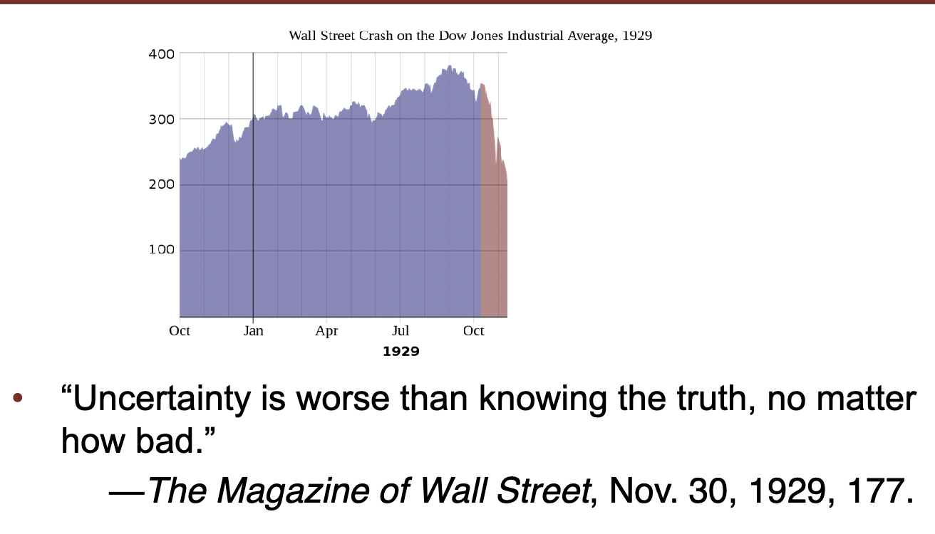
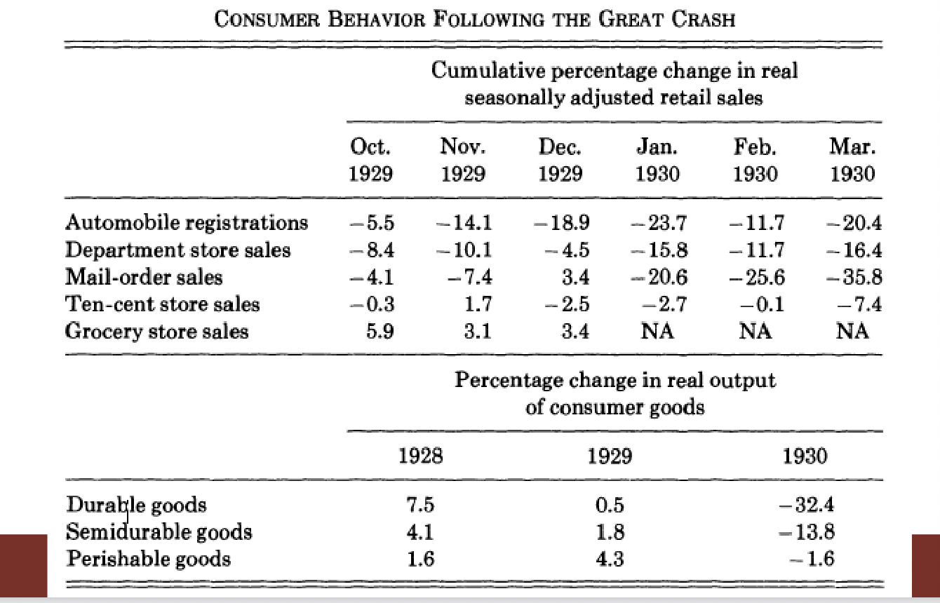
Labor Adjustment Costs:

• Once a negative shock hits, workers must look for new jobs, move to new areas, and sometimes change their wage expectations
• This induces more searching and thus causes more search-related unemployment
• The high cost of reversing job decisions can lead to unemployment
• When faced with uncertainty, many workers will wait, increasing unemployment and magnifying the negative real shock
• Negative shocks come with labor adjustment costs–the costs of shifting workers from the declining sectors of the economy to the growing sectors

Network Effects and Time Bunching:

• Network effects exist where there the value a user derives from a good or service depends on the number of people using compatible products
• With network effects, there’s a positive spillover of consumption
• Network effects are also central in urban economics
• Many activities cluster in location because it pays to coordinate your economic actions with those of others

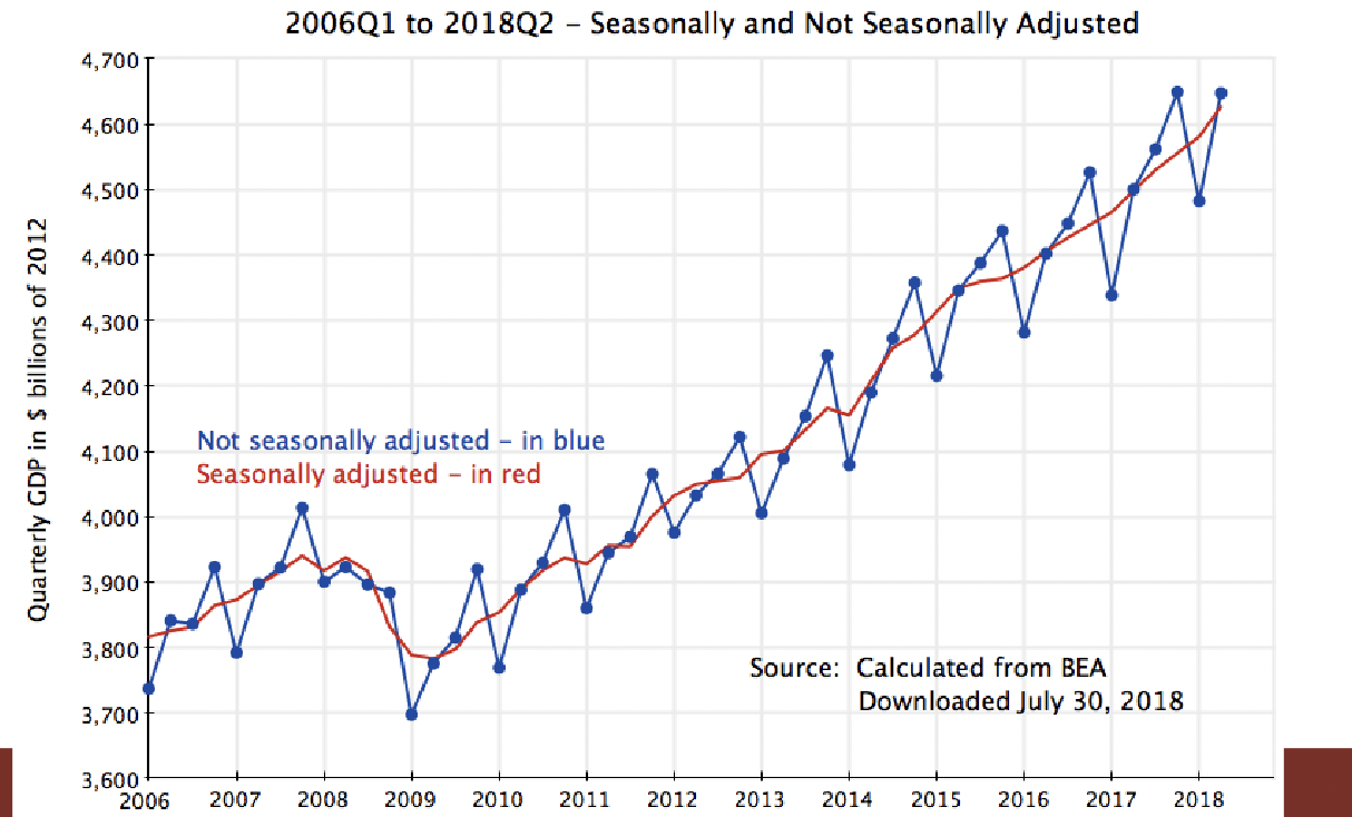
• Network effects also lead to time bunching, the tendency for economic activities to be coordinated at common points in time

- It pays to coordinate your economic actions with those of others

- We often want to invest, produce, and sell at the same time as others

- This clustering of economic activity in time makes buying and selling more efficient

- It also causes shocks to spread through they economy and to spread through time

Collateral Damage:

• Banks are more concerned about downside risk because if a customer does poorly, the bank could lose the entire value of its loan
• If the firm does incredibly well, the bank simply gets its loan back plus interest
• Banks don’t often invest in start-ups or firms with debts that exceed assets
• This behavior amplifies booms and busts for the economy as a whole
• Collateral: A valuable asset that is pledged to a lender to secure a loan. If the borrower defaults, ownership of the collateral transfers to the lender
• Collateral shock: A reduction in the value of collateral. Collateral shocks make borrowing and lending more difficult
• During a boom, asset prices go up and firms have cash flow
• Banks thus become willing to approve more loans, making the boom even bigger
• In a downturn, asset prices fall, cash flow is reduced, and firms have lower net worth

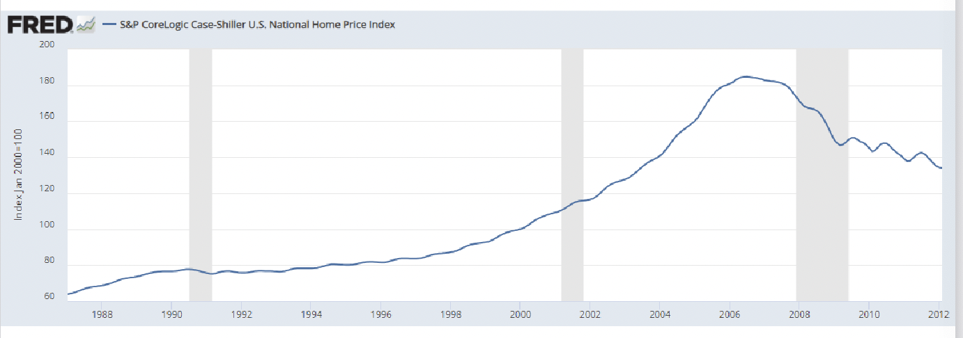
• This price reduction can have a cascading effect as it renders many asset-holders insolvent
• An owner’s equity in an asset is equal to the assets value minus debt associated with it (E = V - D)

- A house worth $400,000 with 10% down and a mortgage of $360,000:

Equity = $400,000 - $360,000 = $40,000

- If the house’s value dropped by $50,000:

Equity = $350,000 - $360,000 = -$10,000

- That is, this asset price reduction rendered the homeowner insolvent–having liabilities exceeding his or her assets

The 2007-2008 Financial Crisis:

• Before the 2007-2008 financial crisis banks “securitized” mortgage loans–bundled them together and sold as financial assets

- The seller of a securitized asset gets cash

- The buyer gets a stream of future payments

• This created a moral hazard for lenders who dumped, bad loans on unsuspecting investors around the world
• The home-price cash left many of the institutions holding these mortgage-backed securities potentially insolvent
• It wasn’t always clear who owned what or who faced the worst losses from failed mortgages
• Credit markets thus froze up with investors becoming unwilling to extend short-term funding to shadow banks
• This led to a fire sale–the vicious circle in which the forced sale of a financial asset drives down the price of related assets, forcing more sales, further driving down the price

Collateral Damage:

• Real shocks and aggregate demand shocks can reinforce and amplify each other
• When the nominal owner of a property doesn’t have much equity in the property, very often he or she doesn’t do a good job taking care of the property
• When the bank itself is “underwater” or nearly so, the bank managers don’t do a very good job of taking care of the bank
• The net result: When asset prices fall, there is a lot of collateral damage

Takeaways:

• At least five factors amplify economic shocks:

1. Labor supply and intertemporal substitution
2. Uncertainty and irreversible investment
3. Labor adjustment costs
4. Time bunching and network effects
5. Collateral shocks

Review:

Unemployment:

The Working Age Population includes:

• 16+
• Civilian
• Noninstitutionalized

Labor Force:

• Employed
• Any amount of hours
• Within working age population

Unemployed:

• 16+
• Civilian
• Non-institutionalized
• Not working but actively looking for work

Unemployment Rate:

Unemployed/Labor Force = Unemployed/Unemployed + Employed

Labor Force Participation Rate:

Labor Force/Working Age Population

Limits of Unemployment Rate:

• Doesn’t account for underemployment (either involunarily part time workers/working not as much as they’d like to be, or not feeling utilized to their full potential with their job)
• Discouraged workers (workers who have given up looking for work but still would like a job

Types of Unemployment:

• Frictional: Ordinary difficulties of matching employer to employee
• Structural: Long term from either a large economy wide shock or labor market policies (policies that discourage hiring people in the short term)
• Cyclical

Natural Unemployment Rate: Tells how well the economy is functioning independent of the business cycle. This is found from adding the frictional and structural unemployment

Inflation:

• General increase in prices, the average price levels
• Pi-P2-P1/P1 x 100

Consumer Price Index:

• Multiply the price for year 1 by the quantities to find the total costs, then multiply the prices from year 2 by the quantities. The ratio between these would give us the CPI for

that year

• Based on what consumers consume

GDP Deflator:

• Nominal GDP/Real GDP x 100
• The percentage increase in prices since the base year

PPI:

• Based on what producers sell
• Increase and grows
• Costs of doing business

Real Price:

Real price = nominal pricet x Po/Pt

• Example: 10,900 x (304.7/29.6) = 112,203
• Example Price of a cell phone: If a phone in 2024 costs $140, its real price in 1985 would be: 140 x (107.6/304.7) = 49.44

Quantity Theory of Money:

• Mv (nominal GDP) =PYr (nominal GDP)
• Money times velocity = Price level times real GDP
• Output comes from the level of technology, physical capital, and labor
• Real interest rate on any asset= nominal interest rate - inflation

R = i-pi (Fisher effect)

• Fisher Effect: Borrowers want a return that will be somewhat related, and the nominal interest rate should equal the real interest rate plus negative inflation. When there is a big increase in expected inflation, there’s going to be an increase in the nominal interest rate
• If the inflation ends up being lower than expected, there will be a higher rate of inflation on those loans
• Inflation can cause a redistribution because taxes tend to be seen on nominal returns not on real incomes. After tax, real returns need to reflect: nominal return after tax = (1- tax rate) times the nominal rate and real rate of return after tax = inflation rate after return - pi
• Dynamic QTM:

M+v=P+Yr

Inflation + real growth = adds up to spending growth. This is used as the basis of the aggregate demand curve

LRAS is not affected by the price level at all

Depends on money growth rate (must be permanent) or velocity growth rate (tend to be temporary)

Unit 4:

Chapter 15 Notes:

The U.S. Money Supplies:

• Money is a widely accepted means of payment and serves as a quick and efficient way of making small transactions.
• The most important assets that serve as means of payment in the United States today are:

1. Currency-paper bills and coins

• Currency is coins and paper bills held by people and nonbank firms.
• U.S. dollars are used in other countries like Panama, Ecuador, El Salvador, and the Republic of Palau

1. Total reserves held by banks at the Fed

• The means of payment you probably don’t have personal experience with, but total reserves play a very important role in the financial system
• All major banks have accounts at the Federal Reserve System (accounts that they use for trading with other major banks and for dealings with the Fed itself)

1. Checkable deposits–your checking or debit account

• Deposits that you can write checks on or can access with a debit card
• The sorts of deposits we use most often in making daily transactions
• Also called demand deposits because you can access this money on demand

1. Savings deposits, money market mutual funds, and small-time deposits

• The largest means of payment are savings accounts, money market mutual funds, and small time deposits
• Each of these components can be used to pay for goods and services, but typically with a little extra work or trouble
• Payment from a savings account can be made by first transferring the money to a checkable account. A money market mutual fund invested in relatively safe short-term debt and government securities
• Small time deposits cannot be withdrawn without penalty before a certain time period has elapsed, usually six months or a year
• Liquid asset:

- An asset that can be used for payments or, quickly and without loss of value, be converted into an asset that can be used for payments.

- The more liquid the asset, the more easily it can serve as money.

- Currency is usually the most liquid asset (currency can be spent anywhere); checkable deposits and reserves are also very liquid, since they can also be spent easily and they can be turned into currency without loss

- Money market mutual funds and time deposits are less liquid since sometimes it takes time to turn these assets into currency or checkable deposits.

- The money supply can be defined in different ways depending on exactly which kinds of liquid assets are included in the definition

• The monetary base: Currency and total reserves held at the Fed
• M1: Currency plus checkable deposits
• M2: M1 plus savings deposits, money market mutual funds, and small time deposits
• The Fed has direct control only over the monetary base. The Fed can increase bank reserves, but if the banks aren’t lending, the increase in reserves won’t do much to increase aggregate demand
• The central bank tried to use its control over MB to influence M1 and M2, but there are many other influences on M1 and M2 so each monetary aggregate can shrink or grow independently of others

Fractional Reserve Banking, the Reserve Ratio, and the Money Multiplier:

• Fractional reserve banking: A system in which banks hold only a portion of deposits in reserve, lending the rest
• Competition among banks to attract funds means that if the bank lends out your money and charges 5% interest, the bank must share some of that return with you. They will pay, for example, 2% for providing the money that they lend. You don’t get the full 5% return because the bank is bearing the risk on the loans, plus paying the costs of making the loans and monitoring the loan borrowers
• Banks balance benefits and costs and thus decide the ratio between reserves and deposits
• Reserve ratio: The ratio of reserves to deposits. If $1 in cash is held in reserve for every $10 of deposits, the reserve ratio is 1/10
• Money multiplier: The amount of money supply expands with each dollar increase in reserves; MM = 1/RR where RR is the reserve ratio. The money multiplier is the ratio of deposits to reserves, or in this case, 10.
• The Fed can create new money at will either by printing it or by adding numbers to bank accounts held at the Fed
• Example: Your bank account has been credited with an additional $1,000. Your bank now has $1,000 in extra reserves, so in order to restore its reserve ratio to 1/10, your bank will want to keep $100 in reserve and make additional loans of $900, lending that amount to sam. Now Sam’s bank has an extra $900, and it doesn’t want to keep all of that in reserves, so it keeps $90 and lends the rest, keeping its reserve ratio at 1/10 and so on and so on. This process becomes a ripple effect as one bank increases its loans, leading to another bank doing the same, etc.
• If banks want a reserve ratio of 1/10, then when the Federal Reserve increases reserves by $1,000, deposits must ultimately increase by $10,000. The money multiplier is the inverse of the reserve ratio, or 10. Deposits eventually increase by the increase in reserves multiplied by the money multiplier.
• If the money multiplier is 10 for example, then an increase in reserves of $1,000 will lead to an increase in deposits of $10,000.
• Change in money supply = change in reserves x money multiplier (MS = Reserves x MM

How the Fed Controls the Money Supply:

Two Major tools the Fed uses to control the money supply-

1. Open market operations–the buying and selling of (usually) short-term U.S. government bonds on the open market
2. Paying interest on reserves held by banks at the Fed

Open Market Operations:

• The Fed’s increase in the money supply spreads throughout the economy. And if the Fed wanted to reduce the money supply, it could sell items it had previously bought, like government bonds
• Treasury bills or T-bills: Short-term bonds
• Government bonds can be stored and shipped electronically and the market for government bonds is liquid and deep, which means that the Fed can easily buy and sell billions of dollars’ worth of government bonds in a matter of minutes:
• Open market operation: The buying and selling of government bonds by the Fed.
• Banks will make additional loans, the loans will in turn be used to buy goods and pay wages, and people will deposit some of these payments into other banks, which will now also be able to make more loans
• The purchase of bonds by the Federal Reserve leads to a ripple process of increasing deposits, loans, and so forth
• The sixe of the money multiplier is not fixed. It is the inverse of the reserve ratio, and the reserve ratio is determined by banks
• When banks are reluctant to lend the money multiplier will be low and a change in the monetary base need not change the broader monetary aggregates much at all
• Even though the Fed controls the monetary base, the Fed may not know how much or how quickly changes in the base will change loans and the broader measures of the money supply
• The federal reserve can increase or decrease reserve banks by buying or selling government bonds, the increase in reserves boosts the money supply through a multiplier process, and the size of the multiplier is not fixed but depends on how much of their assets the banks want to hold as reserves

Open Market Operations and Interest Rates:

• When bond prices go up, that is another way of saying interest rates go down, and when bond prices go down, that means interest rates go up. When the Fed buys or sells bonds, it changes the monetary base and influences interest rates at the same time
• When the Fed buys bonds, it increases the demand, which pushes up the price of the bonds
• Interest rates are determined in a broad market through the supply and demand for loans

The Fed Controls a Real Rate Only in the Short Run:

• Lending and borrowing decisions depend on the real interest rate, the interest rate after inflation has been taken into account
• Federal funds rate: The overnight lending rate from one major bank to another
• Instead of deciding to increase the money supply by $50 billion, the Fed might decide to reduce the Federal Funds rate by a quarter of a percentage point–the Fed will then buy bonds until the Federal Funds rate drops by a quarter of a point

Quantitative Easing:

• The Fed dramatically increased the supply of reserves–so much that it pushed the Federal Funds rate very close to zero
• Zero lower bound: Situation in which the Federal Funds rate is close to zero
• In 2009, the Fed pushed the Federal Funds rate to near the zero lower bound, and still the economy wasn’t bomming
• Quantitative easing: Situation that occurs when the Fed buys longer-term government bonds or other securities

Payment of Interest on Reserves:

• In the midst of the financial crisis, the Federal Reserve focused on a payment of interest on reserves to control the money supply
• Before October 2008, the supply of reserves and the Federal Funds rate were tied closely together. When the Fed increased the supply of reserves the Federal Funds rate would be pushed down, and when the Fed decreased the supply of reserves the Federal Funds rate would be pushed up
• When the Fed pays interests on reserves, it puts a floor on the Federal Funds rate because no bank would want to lend to another bank at a rate that was less than what they could get just by holding onto their reserves
• Starting in 2008, excess reserves increased from 2 billion to 2.8 trillion. Even though the Fed pays only a very low interest rate on reserves, banks are willing to hold many reserves because interest rates in the wider economy are also close to zero
• The Federal Reserve conducts monetary policy by changing the demand for reserves
• They raise the rate of interest they pay on reserves, and that increases the demand, also placing upward pressure on other short-term interest rates
• Liquidity trap: Situation in which interest rates are close to the zero lower bound, so pushing them lower is not possible or not effective at increasing aggregate demand.

The Federal Reserve is the Lender of Last resort:

• Insolvent institution: A bank or institution whose liabilities are greater in value than its assets.
• Illiquid asset: An asset that cannot be quickly converted into cash without a large loss in value; perhaps because the asset is difficult to value and it takes time to find the right buyer
• Banks establish long-term relationships with their customers
• A bank run can break the continuity necessary to fund long-term projects
• Deposit insurance ensures depositors that even if the bank is insolvent they will still be paid
• Systemic risk: The risk that the failure of one financial institution can bring down other institutions
• At the height of the 2008-2009 financial crisis, the FDIC, and the U.S. Treasury stepped in to support the financial system on an unprecedented scale
• The Fed also extended its lending beyond banks to become the lender of last resort to other financial intermediaries in the commercial paper and asset-backed securities markets
• When individuals or institutions are insured, they tend to take on too much risk
• Moral hazard:Moral hazard increases incentives to double bets to make up for a large loss
• Limiting systemic risk while checking moral hazard is the fundamental problem the Fed faces as a bank regulator. In addition, the financial system has become more complex and intertwined as financial assets are packaged, subdivided, bought, and sold more than every before
• The Fed is trying to steer a course between two problems. If a panic occurs, it may be best to bail out some firms, even bad actors, to protect the system, and yet the promise to bail out firms in a future panish encourages risk taking and increases the probability that a panic will happen in the first place

Aggregate Demand and Monetary Policy:

• Beginning at a, an increase in M shifts the aggregate demand curve outward, moving the economy to point b, where inflation and the real growth rate are higher
• After transition the economy will move to point c with a higher inflation rate but a growth rate given by the fundamentals at the long-tun potential level

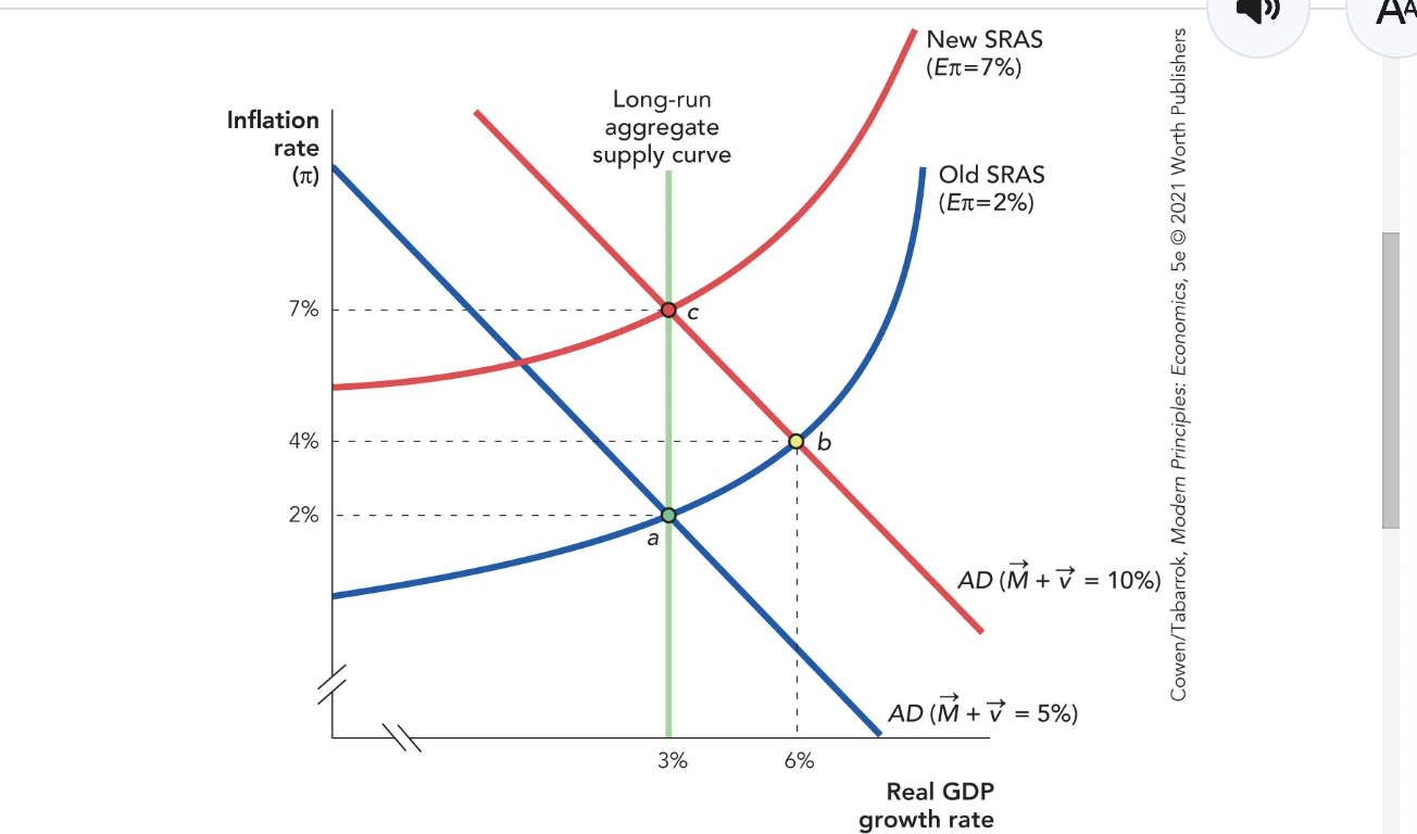
• To estimate the effect of its actions on aggregate demand, the Fed must try to predict and monitor many variables determining the size and timing of the response to its actions
• The Federal Reserve’s power should not be underestimated but increasing or decreasing aggregate demand is not like turning a tap on and off

Who Controls the Fed?

• The Fed has a seven-member Board of Governors, who are appointed by the president and confirmed by the Senate
• Governors are appointed for 14-year terms and cannot be reappointed–this means a single president will rarely appoint a majority of the board
• The Fed has to periodically report to overseers in both houses of Congress
• The Fed is not just one bank but 12 Federal Reserve Banks, each headquartered in a different region of the country
• The Fed is a quasi-private, quasi-public institution
• Each regional bank is a nonprofit with nine directors: Six of these are elected by commercial banks from the region and three are elected by the Board of Governors
• No single president appoints all the governors of the Fed, the governors do not have complete control over Fed policy, the regional bank presidents come from all over the U.S., and they are appoointed by directors who are drawn not just from banking but from a wide variety of fields
• In the financial crisis of 2008, the Fed had to work closely with the Treasury Department
• Political pressures have been put on the Federal Reserve and some chairpersons have been less independent than others
• An independent Federal Reserve is defended by most economists as part of the U.S. system of checks and balances

Takeaway:

• The Federal Reserve is the government’s bank and the bankers’ bank, and it has the power to create money
• The ability to create money, regulate the money supply, and potentially lend trillions of dollars means the Fed has significant powers to influence aggregate demand in the world’s largest economy
• MS = Reserves x MM
• When the government buys securities, the interest rate decreases and that stimulates consumption and investment borrowing

April 8th Notes:

Introduction:

• Through its influence over the money supply, the Federal reserve has more influence over inflation and aggregate demand than any other institution
• Shifts in aggregate demand can greatly influence the economy in the short run
• This chapter looks at the Federal Reserve System and the tools it uses to influence the money supply, aggregate demand, and the economy

Functions of Money:

• Medium of exchange → Money is used to buy goods and services
• Unit of account → Money is a common unit used to measure economic value
• Store of value → Money can be saved

Before the Fed:

Like most early moderns, colonial Americans faced “the big problem of small change:

• “Small”

- Small enough for everyday transactions

• “Change”

- Convertible to legal tender with more than local circulation

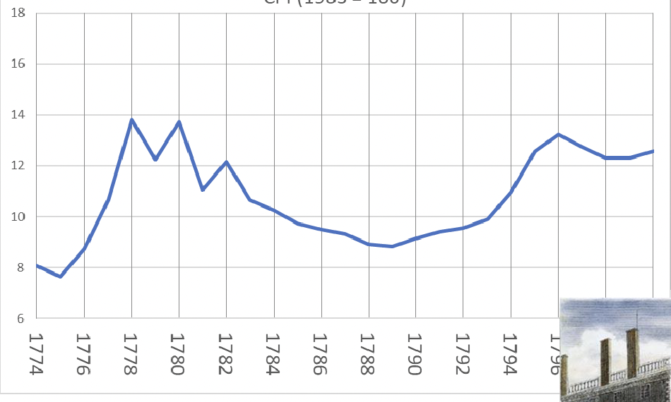
• Hamilton’s Report on Public Credit
• First Bank of the U.S. (1791-1811)

- 20-year charter

- ⅕ of shares owned by th efederal government

- Remaining ⅘ privately owned

- Fiscal agent of the U.S.

- Commercial Banking

• Second Bank of the U.S. (1816-1836)

- Some business model as 1st

• Both also regulated the money supply like a modern central bank
• After the S.F. earthquake, railroad-rate regulation, and an antitrust ruling against Standard Oil weaken markets, a failed October-1907 attempt to corner united Copper Company stock brought the collapse of NY’s 3rd largest trust
• The Knickerbocker Trust Co.’s failure led to a panic, where regional banks withdrew reserves from NY banks
• The result was the Panic of 1907
• J.P. Morgan (1837-1913) pledged millions of his own money and corralled NY’s other leading investment bankers to stave off further fire sales
• Though his actions averted deeper financial disaster, Morgan’s lead role in the Panic of 1907 inspired congressional investigations of this “money trust”

Jekyll Island Meeting, Nov. 1910-

- R.I. Sen. Nelson Aldrich invites five associates on a 10-day “duck hunting trip”

The Aldrich Plan (1910)-

- 15 regional central banks, each governed by boards elected by local bankers

- Regional central banks coordinated by a national board of commercial bankers

- The plan would have created an independent central bank capable of acting as the missing lender of last resort in the Panic of 1907 while providing an elastic currency, but a Democratic house voted it down

Glass-Owen Federal Reserve Act-

• The Wilson Administration’s response to the Aldrich Act
• Feared dominance by bankers and populist challenges
• Maintained much of its model for central banking but brought more federal oversight with the president appointing central board members
• Passed and signed into law on Dec. 23, 1913

What is the Federal Reserve System?

• Since 1913, the Federal Reserve has been America’s central bank
• The Fed is the government’s bank

- Maintains the U.S. Treasury account

- Manages government borrowing through U.S. Treasury bonds, bills, and notes

• The Fed is also the bankers’ bank

- Regulates banks and lends them money

- Manages the nation’s payment system

- Protects financial consumers with disclosure regulations

• The Fed’s most important job is to regulate the U.S. money supply

- It has the power to print money

- It can also add to the monetary base by adding reserves to bank accounts held at the Fed

- This new money can be given away or lent out in a way that increases aggregate demand

• In so doing, the Fed can also shape interest rates
• Comprised of the Board of Governors in Washington D.C., and 12 Federal Reserve distinct banks scattered across the country

What is Money?

• Money is a widely accepted means of payment
• The most important assets that serve as means of payment in the United States today:

- Currency–paper bills and coins

- Total reserves held at the fed

- Liquid deposits–primary checking and savings accounts

- Money market mutual funds and small time deposits

Who Controls the Fed?

• The Fed has a seven-member Board of Governors who are appointed by the president for 14-year terms and confirmed by the Senate
• The president appoints one of the members of the Fed’s Board of Governors as its chair
• After being confirmed by the Senate, the appointee serves as chair for a four-year term
• The Fed is made up of 12 Federal Reserve Banks, each headquartered in a different region of the country
• The Federal reserve is one of the most independent agencies in the U.s. government
• Its considerable power is dispersed.

- No one president appoints all the governors

- The governors do not have complete control over Fed policy

- The governors do not have complete control over Fed policy

- The regional bank presidents come from all over the United States

- Regional bank presidents are appointed by directors from many sectors, not just banking

Whatis not a function of the Federal Reserve: Lending money to consumers

Lender of Last Resort:

• Under certain conditions, depositors may panic and then all try to withdraw their money at once, causing a bank run
• Depositors can’t tell whether the bank is really insolvent or just illiquid

- An insolvent institution has liabilities that are greater than its assets

- A bank with illiquid assets hold assets that cannot be quickly converted into cash without a large loss in value. A bank may be liquid but not insolvent

• That’s where deposit insurance and the Federal Reserve come in–to prevent solvent but illiquid institutions from facing bank runs
• Traditionally, the Fed lent to solvent but illiquid banks
• In a panic, the Fed may also lend to insolvent institutions to limit systemic risk

- Systemic risk (aka systemic uncertainty) is the hazard that the failure of one financial institution can bring down other institutions.

• During the 2008 financial crisis, the Fed bought trillions of dollars’ worth of longer-term government bonds and mortgage-backed securities, lending more than $1 trillion to financial intermediaries
• When individuals or institutions are insured, they tend to take on too much risk
• Institutions that policymakers have deemed “too big to fail” have too little incentive to make responsible financial investments, bringing a problem of moral hazard

- Moral hazard in the financial system occurs when banks and other financial institutions take on too much risk, hoping thatthe Fed and regulators will later bail them out

• The Fed thus faces a trade-off between limiting systemic risk and checking moral hazard

Money:

• A widely accepted means of payment
• Businesses transfer money by wiring money from one bank to another. Likewise, consumers use debit cards or transfer services such as Venmo

- Banks are instructed to transfer money to teh seller’s bank

• All major banks have bank accounts at the Federal Reserve (the Fed)
• When Bank A makes a payment to Bank B, it authorizes the Fed to deduct the money from its account at the Fed and credit the Bank B’s account at th eFed
• Bank accounts at the Fed are often called total reserves and play an important role in the financial system.
• The Fed controls two major means of payment in the United States: currency and reserves held at the Fed
• The Fed also has the power to create money

- It doesn’t have to literally print money since it can add reserves to bank accounts held at the Fed

- This new money can be given away or lent out in a way that increases aggregate demand

• Currency and total reserves are the two final means of payment, but are not the only widely accepted menas of payment
• The most important assets that serve as means of payment in the U.S. today:

- Currency–paper bills and coins

- Total reserves held at the Fed

- Liquid deposits–primary checking and savings account

- Money market mutual funds and small time deposits

• Currency is coins and paper bills held by people andnonbank firms.
• Total U.S. currency amounts to about $5,200 per person.
• Quite a bit of U.S. cash is used in other countries.
• Panama, Ecuador, El Salvador, and some other countries use the U.S. dollar as their official currency.
• Dollars are also used unofficially in unstable countries as a means of preserving wealth.
• Total reserves play an important role in the financial
• system.
• All major banks have accounts at the Federal Reserve, which they use for trading with other banks and theFed itself.
• Electronic claims, though not actually currency, can be converted into currency if the bank wishes.
• Checkable deposits are deposits that you can write checks on or access with a debit card.
• They are the deposits used most often in making daily transactions.
• They are also called demand deposits because you can access this money “on demand.”

Chapter 16 Notes:

The Negative Real Shock Dilemma:

• A very difficult case for monetary policy is when the economy is hit by a negative real shock such as a rapid oil price increase
• A negative real shock shifts the long-run aggregate supply curve to the left, moving the equilibrium from point a to point b

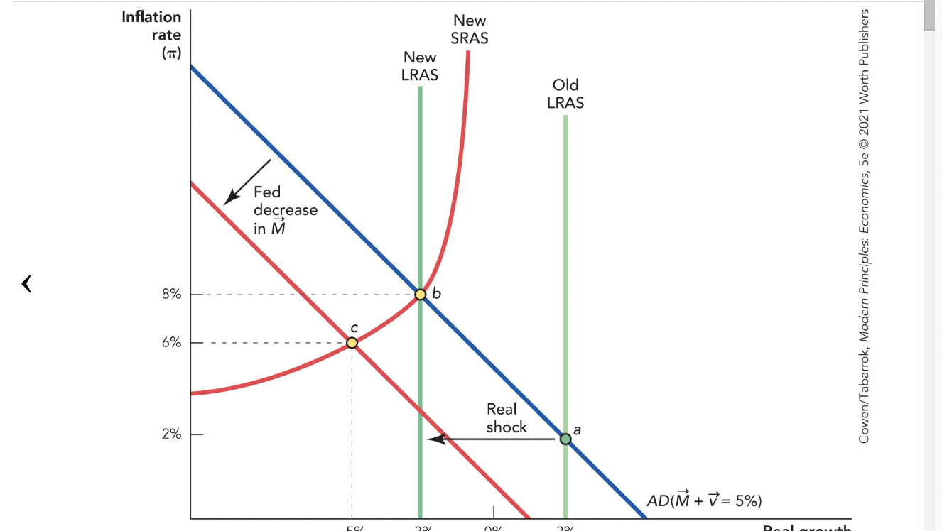
• One approach for monetary policy is to focus on the inflation rate, which has jumped from 2% to 8%. A decrease in inflation occurs due to a decrease in M
• The Federal Reserve often responded to supply shocks, such as an oil shock, by decreasing M and reducing aggregate demand. This menas taking the AD curve and shifting it farther back to the left through the use of monetary policy
• In the figure, the new equilibrium is at point c. The reduction in M reduces the inflation rate from 8% to 6%, but also reduces economic growth and by more than the supply shock alone would have done.
• The Federal Reserve can increase aggregate demand by increasing the money growth ate, but, when the economy is facing a negative real shock, it is less productive than at other times, due to the real shock
• Central bankers are more likely to believe that a central bank should respond to a respond to a negative real shock by increasing aggregate demand
• An increase in M will not move the economy back to point a. Instead, most of the increase in M will show up in inflation rather than in real growth so the economy will shift from point b to point c, as shown in the graph with a much higher inflation rate and a slightly higher growth rate

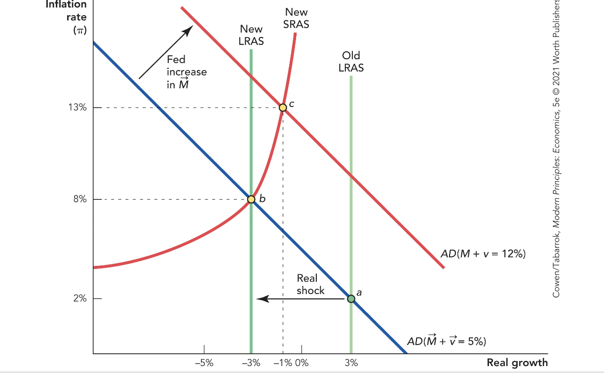
• Although an increase in M may increase the growth ate a little, the inflation rate increases by a lot and, higher inflation now can cause serious problems later
• If the inflation rate gets too high, the Fed has to reduce inflation, thereby creating a lot of unemployment
• Real shocks are often accompanied by aggregate demand shocks, so the figures are considerably simplified
• Social distancing and lockdown orders created a recession that monetary policy couldn’t fix
• The Federal Reserve looks at real-time data
• With a real shock, the central bank has to choose between too low a rate of growth and too high a rate of inflation

When The Fed Does Too Much:

• The Fed has considerable power to influence aggregate demand but, power is constrained by uncertainty and by an inability for anyone to fully understand the complexity of the economy
• A number of economists have argued that Federal Reserve policy in 2001-2004 contributed to the housing boom and eventual bust that led to the financial crisis in 2007-2008
• Many factors contributed to the financial crisis, including too much leverage and irrational exuberance
• The financial crisis and the Fed’s role in it are highly debated topics among economists and a consensus has not yet been reached
• In the late 1990s, the American economy was the envy of the world. Economic growth was strong and the unemployment rate was low, even dipping below 4% in 2000
• The unemployment rate continued to increase even after the recession had officially ended
• From a rate of 4% in 2000, unemployment increased during the recession to 5.5% and then kept increasing until it peaked at 6.3% (almost a 50% increase) in June 2003
• To combat the high unemployment rate after 9/11, the Fed tried to increase aggregate demand through expansionary monetary policy
• The Federal Funds rate is a short-term interest rate that is largely under the control of the Federal Reserve. During the recession, the Fed pushed down the Federal Funds rate from about 6.5% in 2000 to 2% at the end of 2001 when the recession ended
• From mid-2003 to mid-2004, the Fed held the Federal Funds rate at 1%, an extraordinarily low rate
• The low Federal Funds rate helped to make credit cheap throughout the economy
• A bubble arises when asset prices rise far higher and more rapidly than can be accounted for by the fundamental prospects of the asset. Prices are instead driven by shifts in market psychology and successive waves of irrational exuberance. Cheap, easy credit makes it easier for investors to operate and intensify bubbles.
• The low interest rates are, in essence, signalling to market participants that credit is easy and it is a good idea to borrow money
• Distorted price signal: Arises when government policy moves in a manner that encourages investors to take risks
• The Fed began to raise interest rates in mid-2004 but rates remained very low until at least mid-2005. In 2006 housing prices peaked, and by 2007 were in free fall
• Because housing prices peaked, they would soon after fall: This reduced aggregate demand, contributed to a freezing up of financial intermediation as banks and others took huge losses on poor investments in mortgage securities
• Since bank lending is a main generator of M1 and M2, thisi menas lower rates of growth for the money supply. By the fall of 2008, the growth rate was negative, meaning that that the American economy was shrinking

Dealing with Asset Price Bubbles:

• The economy had quickly recovered from the much larger drop in stock prices during the tech bubble that ended with the recession of 2001
• It’s not always easy to identify when a bubble is present. If everyone knew it was an unsustainable bubble, then all should have invested accordingly and bet against the bubble, thereby enriching themselves and also stopping the bubble in the first place
• Monetary policy is a crude means of popping a bubble. It can influence aggregate demand, or target credit markets at the aggregate level, but monetary policy can’t push the demand for housing down and keep the demand for everything else up. Thus, popping a bubble means reducing th growth rate of GDP for the broader economy as a whole
• In addition to monetary policy, the Fed does have the power to regulate banks and it probably could have restrained some of the “subprime,” no-questions-asked mortgages that were sold during the boom and later went into default
• Monetary policy is difficult in the worst of times and it’s not easy in the best of times

Rules vs. Discretion:

• The possibility of the “too little and “too much” responses, or in othe rwords the imperfections of monetary policy, has led to a debate over rules versus discretion when it comes to monetary policy
• Ideally, monetary policy tries to adjust for shocks to aggregate demand, but it is often debated whether these adjustments are effective in reducing the volatility of output
• If Fed responds too often in the wrong direction or with the wrong strength, GDP volatility will increase rather than decrease
• A typical monetary rule would set target ranges for the monetary aggregates like M1 or M2 or for the rate of inflation. Nobel Prize winner Milton Friedman, for example, advocated a strict rule in which the money supply would grow by 3% a year every year, since the U.S. economy has a long-run growth rate near 3%.
• A monetary rule works best only when v, monetary velocity, doesn’t change rapidly. To see one problem with a monetary rule, the quantity theory of money can be used (Mv=PYr), where M is the money supply, v is velocity, P is the price index, and Yr is real GDP
• A monetary rule says keep M constant, but that menas that the Fed must ignore changes in v.
• If M is constant and v falls, then either P must fall or Yr must fall. Since prices are sticky, the usual outcome is that both P and Yr fall, and a fall in Yr means a recession
• The nominal GDP rule: Keeps Mv constant. If Mv doesn’t change or grows smoothly, then so does PYr, and that would be ideal
• A nominal GDP rule would have required the Federal Reserve to increase M by as much as it takes to keep nominal GDP growing at around 5% a year.
• If the Fed had followed a nominal GDp rule, the recession of 2008 would have been much milder
• Proponents of a nominal GDP rule say the Fed did too little, too late. In this view, if the Fed had acted sooner and given the markets clearer guidance, then v would have stayed higher and the Fed could have more easily returned nominal GDP to its trend.

Takeaway:

• The Fed has some influence over the growth rate of GDP through influence over the money supply and thus AD
• An increase in M increases AD and a decrease in M decreases AD
• When faced with a negative shock to AD, the central bank can restore aggregate demand through an expansionary monetary policy. Poor monetary policy can decrease the stability of GDP
• If in responding to a series of recessions, the Fed increases M too much, it may find that it later has to contract when inflation becomes too high
• A disinflation goes best when the central bank has some degree of credibility in its attempt to set things right
• A central bank would like low unemployment and low inflation, but it is not always possible to achieve both goals
• Monetary policy is difficult in the worst of times and it’s not easy in the best of times. The Federal Reserve has significant power but that power is not always easy to wield.
• Real shocks and aggregate demand shocks are always mixed and not easy to disentangle

April 10th Notes:

The U.S. Money Supplies:

• The money supply can be defined in different ways depending on which liquid assets are included in the definition

- Liquid assets are assets that can be used for payments or, quickly and without loss of value, be converted into assets that can be used for payments

Three most important definitions of the money supply:

• M1: Currency plus checkable deposits
• M2: M1 plus savings deposits, money market mutual funds, and small time deposits
• The Fed has direct control only over the monetary base. The Fed can increase bank reserves, but if the banks aren’t lending, the increase in reserves won’t do much to increase aggregate demand
• The central bank tried to use its control over MB to influence M1 and M2, but there are many other influences on M1 and M2 so each monetary aggregate can shrink or grow independently of others
• This control is indirect due to fractional reserve banking, which means banks hold only a fraction of their deposits in reserve, lending the rest.
• Thus, there are many other influences on M1 and M2.
• Although M1 and M2 affect aggregate demand, there are also other influences.

Fractional Reserve Banking:

• When money is deposited into an account, the bank holds a fraction of the account balance in reserve and uses the rest to make loans.
• Banks earn a profit on these loans.
• Banks share some of the profit with depositors by paying interest on the money you provide.
• They also provide services like check writing and check clearing
• The law and the Federal Reserve require banks to
• keep some reserves.
• Banks need those reserves to meet depositor demands for currency and payment services.
• Reserves involve opportunity costs: Money held in reserve isn’t being lent, and lending is where banks earn most of their profits.
• Banks balance these benefits and costs when deciding on the ratio between reserves and deposits.
• The monetary base includes: currency and reserves held by banks at the federal reserve

Reserve Ratio:

• The Reserve ratio (RR) is the ratio of bank reserves to deposits.
• If $1 in cash is held in reserve for every $10 of deposits, the reserve ratio is: 1/10=0.10
• The reserve ratio is determined primarily by how liquid banks wish to be

The Reserve Ratio and Money Multiplier:

• The inverse of the reserve ratio is called the money multiplier (MM).
• This Money multiplier (MM) is the amount that the money supply expands with each dollar increase in reserves.
• The money multiplier is the ratio of deposits to reserves. MM = 1/RR.
• In our case:= 10/1=10
• The money multiplier tells us how much deposits expand with each dollar increase in reserves.

Money Multiplier:

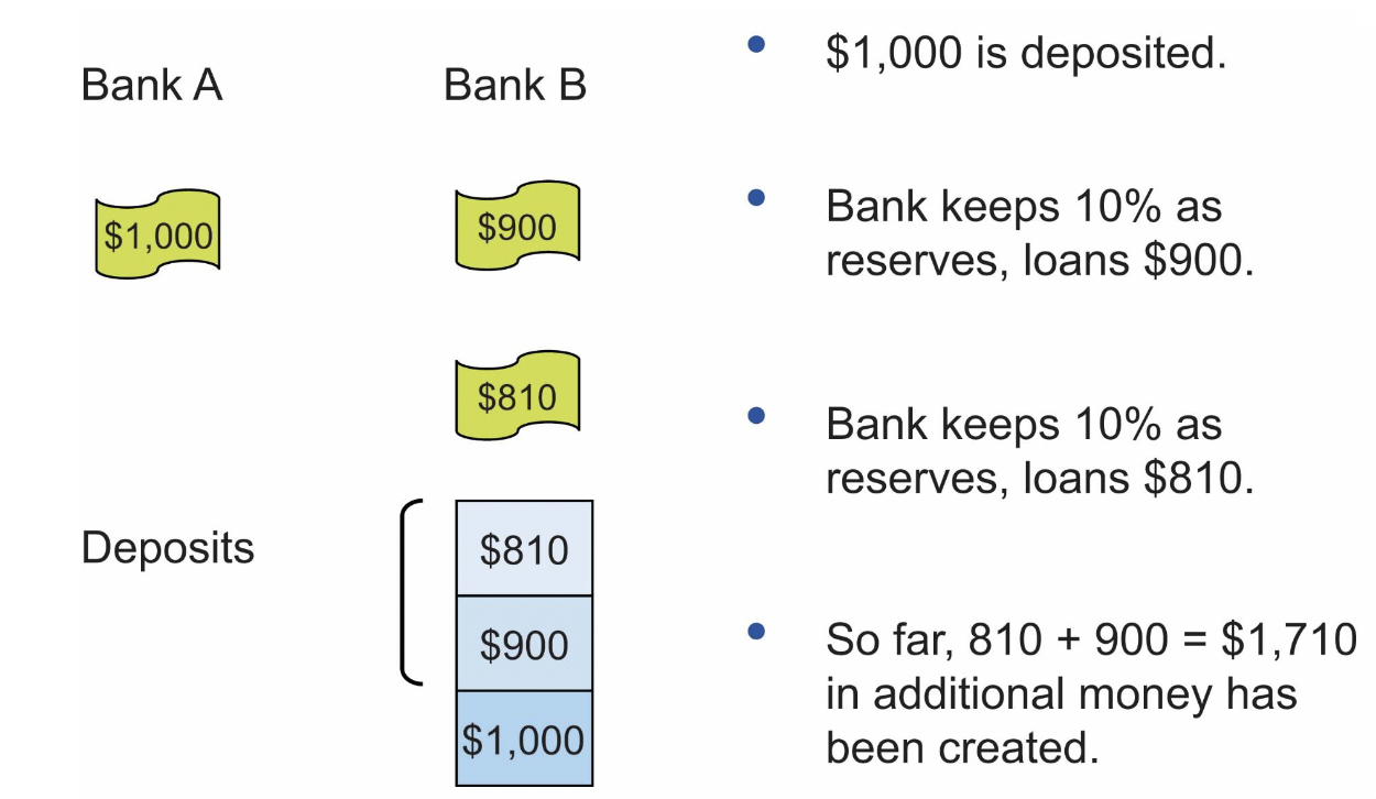
• The process continues until there are no excess reserves to lend.
• With a reserve ratio of 10%, the money multiplier = 1/0.10 = 10.
• The initial $1,000 increase in reserves can expand total deposits (money supply) by:

- Change in reserves × MM = Change in money supply

$1,000 × 10 = $10,000

• If the reserve ratio is 5%, the money multiplier is equal to: 1/0.05 = 20

Controlling the Money Supply:

• The Fed has two major tools to control the money supply:

1. Open market operations

2. Paying interest on reserves held by banks at the Fed

The Fed’s Tools to Change the Money Supply or “Liquidity”

The Fed has three tools to change the supply of money:

1. Open market operations
2. Repurchase agreements (repos)
3. Quantitative easing

Open Market Operations:

• Open market operations occur when the Fed buys or sells government bonds
• The Fed changes the money supply by buying or selling government bonds (T-bills).
• To pay for the T-bills, the Fed electronically increases the reserves of the seller, usually a bank or large dealer.
• With more reserves, the bank can make additional loans, which are used to buy goods and pay wages.
• Reserves are again deposited in a bank.
• The payments for goods and wages are deposited into other banks.
• The new deposits increase the reserves of the banks, which can also make more loans.
• The Fed controls the monetary base, but it does not control how much or how quickly the base will change loans and the money supply.
• The money multiplier is determined by the reserve ratio, which is determined by banks.
• When banks are confident, they will keep their reserves low so the MM will be large.
• When banks are reluctant to lend, the MM will be low and a change in the monetary base will not change the money supply by much.
• When the Fed buys or sells bonds, it changes the monetary base and influences interest rates at the same time.
• When the Fed buys bonds, the demand for bonds increases, pushing up the price of bonds and lowering the interest rate.
• Buying bonds stimulates the economy through higher money supplies and lower interest rates.
• When the Fed sells bonds, the process works in reverse.
• Buying and selling government bonds influences interest rates:

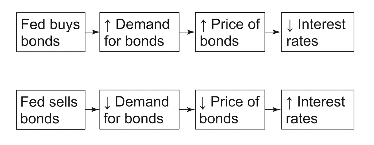
• The Fed usually focuses on the Federal Funds rate, or the interest rate one major bank charges another for an overnight loan.

- It is a convenient signal of monetary policy.

- It responds quickly to actions by the Fed.

- It can be monitored on a day-to-day basis.

• Instead of increasing the money supply, the Fed can buy bonds until the Federal Funds rate drops by the desired amount.
• •The Fed can also increase the Federal Funds rate by selling bonds.

Repos:

• A repo is a temporary open market purchase and adds
• liquid reserves to the banking system.
• From the bank's point of view, a repo is a short-term loan from the Fed to the bank.
• A reverse repo is the opposite

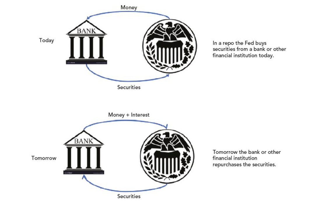
Quantitative Easing:

• During the 2008–2009 recession, the Fed dramatically increased reserves.
• It pushed the Federal Funds rate very close to zero (“zero lower bound”).
• The economy still wasn’t responding.
• The Fed moved to buying and selling longer-term government bonds.
• This kind of quantitative easing is used when the Federal Funds rate is near the zero lower bound.

Quantitative Easing

Quantitative easing:

• When the Fed buys longer-term government bonds or other securities.

Quantitative tightening:

• When the Fed sells longer-term government bonds or other securities

Payment of Interest on Reserves

• Traditionally, the Fed influenced the Federal Funds rate by changing the supply of reserves.
• During the 2008 financial crisis, the Fed wanted to separate these two aspects of monetary policy.

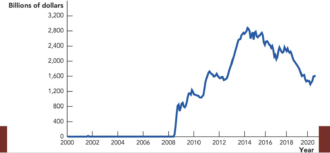
• Paying interest on reserves allowed the Fed to separate the two channels of monetary policy.
• Starting in 2008, it increased excess reserves in the banking system from $2 billion to $2.8 trillion.
• Even though the Fed pays a very low interest rate on reserves, banks are willing to hold lots of reserves because interest rates for other low-risk investments are also close to zero.
• Since then, banks’ accounts at the Fed have grown, representing between $2 trillion and $4 trillion
• There are costs and benefits to holding reserves at the Fed:

– Cost: banks could be using these funds to earn interest by making loans.

– Benefit: Fed pays interest on reserves

• Banks are constantly comparing how much they could earn by lending funds with how much they could earn by holding their funds at the Fed.
• The Fed can choose the interest rate that it pays on reserves to influence lending and aggregate demand:

- If the Fed raises the rate on reserves, banks hold more reserves and make fewer loans, thus decreasing the aggregate demand.

- If the Fed lowers the rate on reserves, banks hold less reserves and make more loans, thus increasing the aggregate demand.

• If the Fed lowers the rate paid on reserves:

– Banks will find it more profitable to lend, increasing the amount of short-term loans

– The lower interest rate encourages consumers and businesses to borrow and invest, which increases spending.

• If the Fed raises the rate paid on reserves:

– Banks will find it less profitable to lend, decreasing the amount of short-term loans

– The higher interest rate discourages consumers and businesses to borrow and invest, which decreases spending.

The Fed’s Tools:

• Open market operations–the buying and selling of short-term U.S. government bonds. The Fed buys bonds to lower interest rates and expand the money supply, and sells bonds to raise interest rates and contract the money supply.
• Raising or lowering the interest rate paid on reserves. The FEd lowers the rate paid on reserves to decrease reserve demand and expand bank lending, and raises the rate to increase reserve demand and reduce bank lending.
• Quantitative easing–the buying and selling of longer-term U.S. government bonds or other securities. Used to influence longer-term rates directly or to support borrowing and lending in especially distressed markets in a crisis
• Lender of last resort–leading to banks and other financial intermediaries in a crisis to maintain borrowing and lending

April 12th Notes:

Coordinating Expectations:

• The Fed’s final tool is talking
• Talking can help the Fed manage and coordinate expectations

Limits to the Fed’s Powers:

• The Fed can change the interest rate to encourage banks to either increase or decrease lending, but what if banks do not change their lending?
• The Fed must try to predict and monitor:

- How much changes in interest rates affect spending, borrowing, and lending

- How quickly changes in interest rates affect spending, borrowing and lending

- Whether businesses and consumers want to invest and borrow

- If businesses do borrow, will they promptly hire labor and capital, or will they just hold the money as a precaution?

- How will the expectation of people and firms respond to the Fed’s actions? Will the Fed’s actions be regarded as temporary?

The Fed Only Influences Real Rates in the Short Run:

• Remember that money is neutral in the long run—that neutrality includes real interest rates.
• Also recall that an increase in aggregate demand increases the real growth rate only in the short run.
• The long-run neutrality of money, the long-run neutrality of aggregate demand, and the long-run neutrality of the Fed's influence over real interest rates are all different sides of the same "coin."

AD and Monetary Policy:

• The Fed uses monetary policy to influence aggregate demand (AD).
• For example, to increase AD, it can buy bonds in an open market operation.

- This expands the monetary base, increasing deposits and loans by the multiplier process.

- It also lowers short-term interest rates, stimulating investment and consumption borrowing.

- If all goes well, AD will increase.

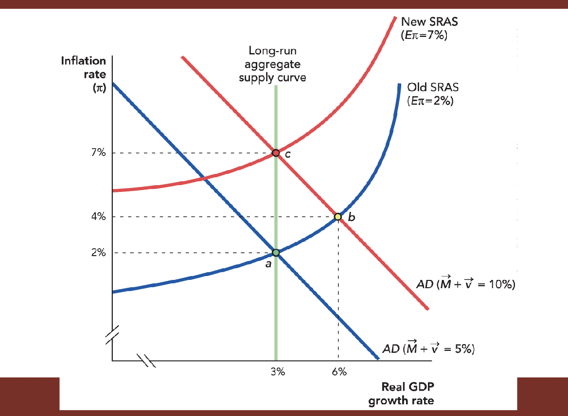
• To estimate the effect on AD, the Fed must try to predict and monitor the following:

– Will banks lend out all the new reserves or only a portion?

– How quickly will increases in the monetary base translate into new bank loans?

– Do businesses want to borrow? How low do short-term interest rates have to go to stimulate more investment borrowing?

– If businesses do borrow, will they hire labor and capital, or just hold the money as a precaution?

Takeaways:

• The Federal Reserve is the government’s bank and the banker’s bank.
• It has the power to create money, regulate the money supply, and potentially lend trillions of dollars.
• This gives it the power to influence aggregate demand in the world’s largest economy.
• The Fed controls the money supply by buying and selling government bonds in open market operations
• The Fed has several tools to influence the aggregate demand.

– Changing the interest rate that it pays on bank reserves

– Open market operations, repos, and quantitative easing

– Acting as the "lender of last resort"

– Coordinating expectations

• It has the most influence over short-term interest rates.

Chapter 16 Lecture Notes:

Introduction:

• In this chapter, we turn to three key practical questions:

1. When should the Fed try to influence aggregate demand

(AD)?

2. When will the Fed be able to influence AD?

3. When will the influence on AD result in higher GDP

growth rates?

Monetary Policy: The Best Case

• Let’s start with an economy that has been growing at 3% with an inflation rate of 7%.
• Suppose it faces a negative shock to AD driven by “animal spirits”—emotions such as fear.

– Consumers become pessimistic, borrowing and spending less.

– Banks lend less, and entrepreneurs cut back on expansions and invest less.

– The negative shock shifts AD to the left, and the growth rate of output declines.

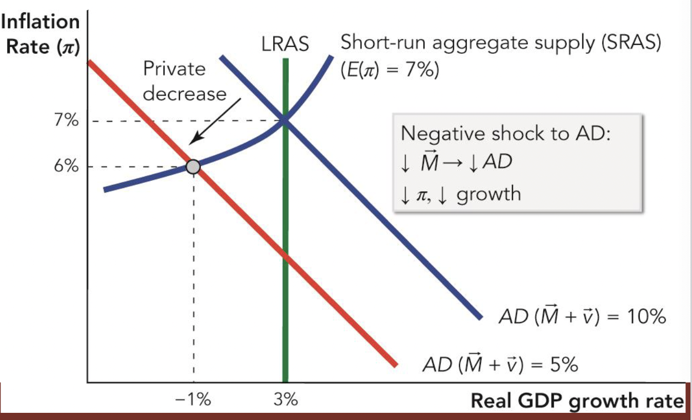
• Eventually, the economy will recover from the negative AD shock.
• Fear recedes and the economy returns to its steady-state growth level.
• However, there is slow growth and increased unemployment, or even a recession in the meantime.
• The Fed can combat this sluggish growth with monetary policy.
• To shift the AD curve back up and to the right, the Fed can:

– Increase the rate of growth of the money supply

– Reduce interest rates and encourage more borrowing

Self-Check:

Which monetary policy can the Fed use to increase AD?

a. increase the rate of growth of the money supply

b. increase interest rates

c. discourage consumer borrowing

Getting Monetary Policy “Just Right” Is Not Easy

• Monetary policy is difficult because:

– The Fed must operate in real time when much of the data about the state of the economy is unknown.

– The Fed’s control of the money supply is incomplete and subject to uncertain lags.

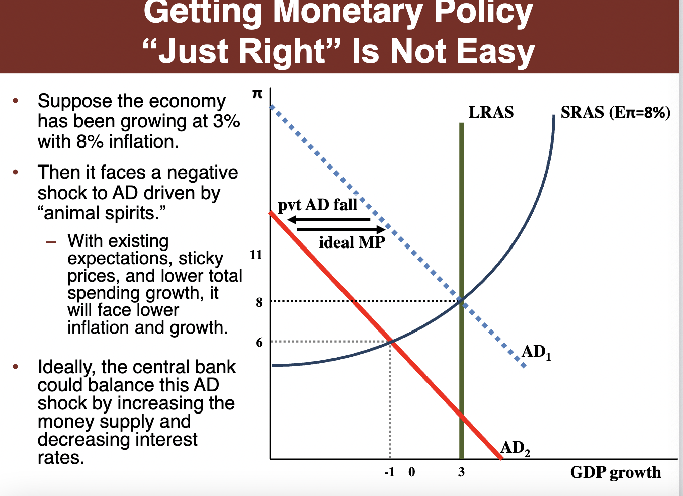
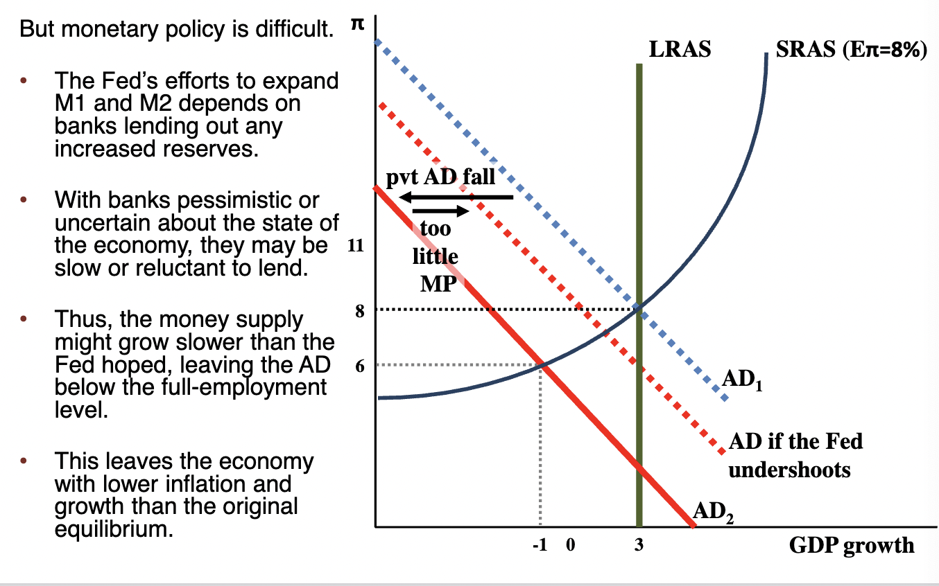
• The Fed can also increase the money supply by more than the cyclical AD decline

- If it does this, it overstimulates the economy

- This leads to a temporary boom, but also higher inflation

• Ideally, the Fed could balance out a decline in aggregate demand by expanding the money supply and lowering interest rates
• But the Fed’s incomplete control over the money supply and limited access to real time date means that

- It might provide too little monetary stimulus to avoid a downward business cycle

- Or it could overstimulate the economy leading to inflation

Decreasing AD:

• Sometimes the Fed overstimulates the economy, increasing AD too much
• Economies may get stuck between continuing a costly rate of inflation or reducing it at the risk of a recession
• Many economists believe the Fed overstimulated the economy in the 1970s, resulting in an inflation rate of 13.5% by 1980
• By 1983, tough monetary policy had reduced the inflation rate to 3%.
• The consequence was a very severe recession with an unemployment rate of a little more than 10%.
• However, the Volcker Shock’s disinflation slowed inflation and provided the foundation for 25 or so years of economic growth.

– Remember that disinflation is a significant reduction in the rate of inflation

• If nominal wage growth outpaces inflation by too much, workers will become expensive, and employers may lay some workers off.
• The key to a less painful disinflation is to increase nominal wage flexibility.
• When they view announcements about tightened monetary policy as credible, workers will be prepared for slower wage growth and will quickly adjust to the inevitable.

– A monetary policy is credible when it is expected that a central bank will stick with its policy.

• A credible disinflation therefore reduces the unemployment effects.

Market Confidence:

• Fear and confidence are some of the most important shifters of aggregate demand.
• When investors are uncertain, they often prefer to wait.
• This is compounded by the bandwagon effect as investors coordinate their actions with others
• One of the Federal Reserve’s most powerful tools is its influence over expectations—namely, its ability to boost market confidence.

– The Federal Reserve influences market confidence by shaping expectations, not by directly changing the money supply.

• For example, uncertainty increased after the terrorist attacks of September 11, 2001.
• If enough people had taken the attacks as a signal to reduce investment, the bandwagon effect or uncertainty could have created a severe recession.
• The Fed increased lending to banks from $34 million to $45.5 billion on September 12.
• This helped stabilize expectations, reduce fear, and raise confidence.

Real Shocks-A Monetary Policy Dilemma:

• A difficult case for monetary policy is when the economy is hit by a negative real shock, such as a rapid oil price increase.
• This shifts the LRAS curve to the left, increasing inflation and decreasing GDP growth.
• A reduction inM reduces the inflation rate, but also reduces economic growth.
• The Fed can increase AD by increasingM
• But the economy is less productive than before, so most of the increase will show up in inflation.
• 
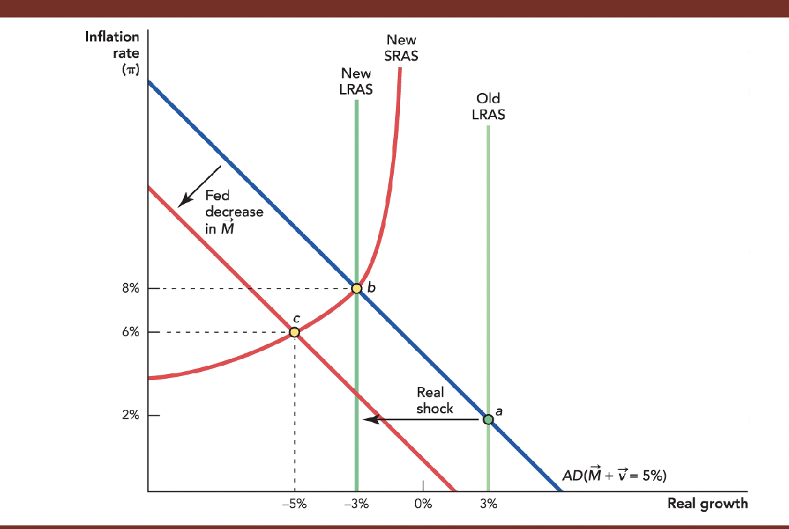
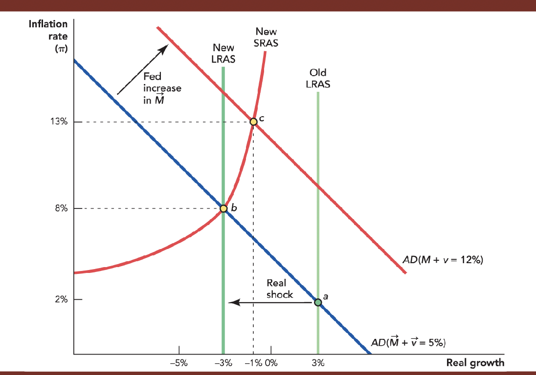
• With a real shock, the central bank must choose between:

- Too low a rate of growth (with a high rate of unemployment)

- Too high a rate of inflation

Self-Check

A negative real shock poses difficulties for monetary policy

because:

a. policymakers can reduce inflation or unemployment,

but not both.

b. increasing the money supply is politically unpopular.

c. increasing the money supply is illegal.

Monetary policy and how real shocks affect it. Negative real shocks can reduce inflation. Sell bonds to decrease money supply and vice versa

April 15th Notes:

Monetary Policy-The Best Case:

• Costaguana has a Solow growth rate of 4%, while its money supply is growing by 10% and its velocity of money supply is growing by 1%. It is going to double in 17.5 years because 70/4=17.5
• With 11% total spending growth and 4% real growth, Costaguana must currently have a 7% inflation rate
• Suppose Costaguana faces a financial crisis, where consumers and entrepreneurs become more pessimistic
• With existing expectations and sticky prices, decreased spending growth will result in decreased real growth and increased unemployment
• Eventually consumers and entrepreneurs’ dears will recede

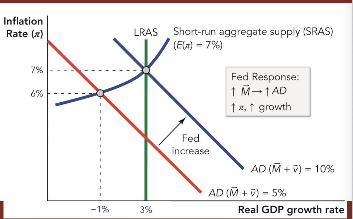
Self-Check: Which monetary policy can the Fed use to increase AD? The Fed can increase the rate fo growth of the money supply to increase AD

Getting Monetary Policy “Just Right” Is Not Easy:

• Monetary policy is difficult because:

- The Fed must operate in real time when much of the data about the state of the economy is unknown

- The Fed’s control of the money supply is incomplete and subject to uncertain lags

• Ideally, the Fed could balance out a decline in aggregate demand by expanding the money supply and lowering interest rates
• But the Fed’s incomplete control over the money supply and limited access to real time data means that

- It might provide too little monetary stimulus to avoid a downward business cycle

- Or it could overstimulate the economy leading to inflation

Decreasing AD:

• Sometimes the Fed overstimulates the economy, increasing AD too much
• Economies may get stuck between continuing
• By 1983, tough monetary policy had reduced the inflation rate to 3%
• The consequence was a very severe recession with an unemployment rate of a little more than 10%
• However, the Volcker Sh
• If nominal wage growth outpaces inflation by too much, workers will become expensive, and employers may lay some workers off
• The key to a less painful disinflation is to increase nominal wage flexibility
• 

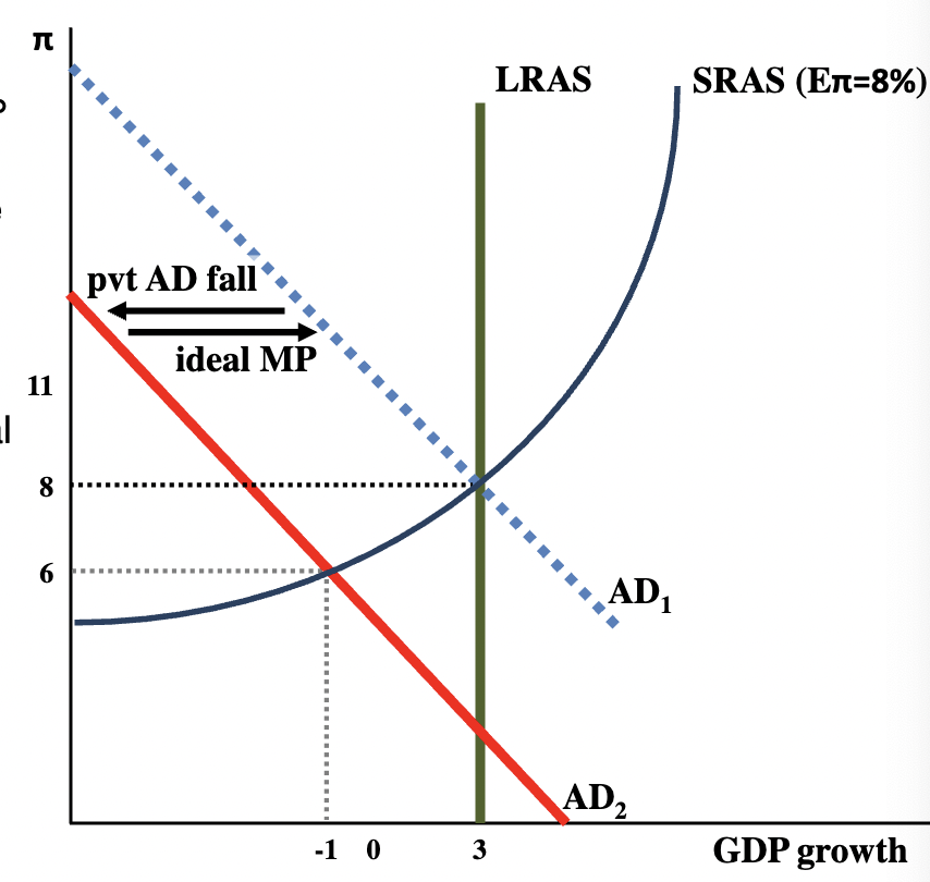
Market Confidence:

• Fear and confidence are some of the most important shifters of aggregate demand
• When investors are uncertain, they often prefer to wait
• This is compounded by the bandwagon effect as investors coordinate their actions with others
• One of the Federal Reserve’s most powerful tools is its influence over expectations–namely, its ability to boost market confidence

- The Federal Reserve influences market confidence by shaping expectations, not by directly changing the money supply

• For example, uncertainty increased after the terrorist attacks of September 11, 2001
• If enough people had taken the attacks as a signal to reduce investment, the bandwagon effect or uncertainty could have created a severe recession
• The Fed increased lending to banks from $34 million to $45.5 billion on September 12
• This helped stabilize expectations, reduce fear, and raise confidence

Real Shocks-A Monetary Policy Dilemma:

• A difficult case for monetary policy is when the economy is hit by a negative real shock, such as a rapid oil price increase
• This shifts the LRAS curve to the left, increasing inflation and decreasing GDP growth
• A reduction in M reduces the inflation rate, but also reduces economic growth
• The Fed can increase AD by increasing M
• But the economy is less productive than before, so most of the increase will show up in inflation
• With a real shock, the central bank must choose between:

- Too law a rate of growth (with a high rate of unemployment)

- Too high a rate of inflation

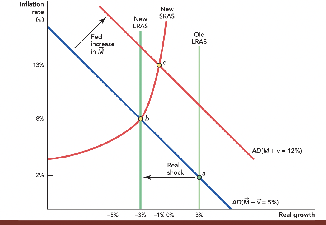
Self-Check:

A negative real shock poses difficulties for monetary policy because:

Policymakers can reduce inflation or unemployment, but not both

When the Fed Does too Much:

• In the late 1990s, U.S. economic growth was strong and unemployment was low
• The 2001 recession didn’t last long, but unemployment continued to increase even after it officially ended
• Three years after the recession ended, the unemployment rate remained near its recession high

- Unemployment kept increasing until it peaked with a 57.5% increase in June 2003 than it was in 2000 with a 4% unemployment rate

• The Fed kept pushing down the Federal Funds rate from about 6.5% in 2000 and held it at 1% until 2004
• The low Federal Funds rate helped to make credit cheap throughout the economy
• It encouraged people to take out more mortgages, bidding up the price of homes
• This fuled a speculative bubble in housing
• Rates remained very low until mid-2005
• In 2006, housing prices peaked; by 2007, they were in free fall
• The real estate crash contibuted to a freezing up of financial intermediation

Asset Price Bubbles:

• It’s easy to say in restrospect that the Fed should have raised rates sooner or more quickly
• There are several problems with this:

1. Few people expected that a fall in housing prices would wreak as much havoc as it did
2. It’s not always easy to identify when a bubble is present
3. Monetary policy is a crude means of “popping” a bubble, because it affects the whole economy

• The Fed has the power to regulate banks
• It could have restrained some of the “subprime,” no questions-asked mortgages that later went into default
• That would have been the best way of limiting the bubble without taking down the broader economy
• Economists have not settled on what to do when asset prices boom

Self Check: Which of the following strategies should the Fed have used to limit the recent housing bubble? The Fed should have regulated subprime mortgages to lmit the housing bubble

Rules v. Discretion:

• Ideally, monetary policy adjusts for shocks to AD, but it is uncertain whether these adjustments are effective in reducing the volatility of output.
• Some economists believe the Fed should follow a consistent policy and not try to adjust to every aggregate demand shock.
• A typical monetary rule would set target ranges for the monetary aggregates like M1 or M2, or for the rate of inflation.
• A monetary rule works best only when v, monetary velocity, doesn’t change rapidly.
• If M is constant and v falls, then either P must fall or Y must fall.
• Since prices are sticky, the usual outcome is that both P and Y fall, and a fall in Y means a recession.
• Other economists have suggested a nominal GDP rule: Keep Mv constant (or growing at a constant rate).
• If Mv doesn’t change or grows smoothly, then so does PY, and that would be ideal

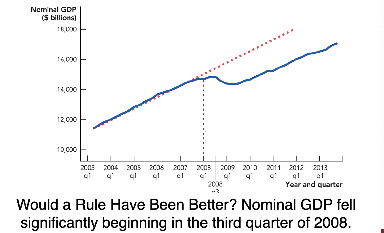
• If the Fed had followed a nominal GDP rule, the recession of 2008 would have been much milder.
• The Fed did not increase M enough to make up for a fall in v, even though the monetary base doubled between August and December 2008.
• Whether the Fed should have or could have kept nominal GDP on track continues to be debated.

April 17th Notes:

Rules vs. Discretion:

• Ideally, monetary policy adjusts for shocks to AD, but it is uncertain whether these adjustments are effective in reducing the volatility of output
• Some economists believe the Fed shouldn’t try to adjust to every aggregate demand shock but should instead follow a consistent policy

- Targeting monetary aggregates like M1 or M2, or for the rate of inflation

- Or targeting a constant NGDP (Mv) or NGDP growth (M+v)

Chapter 18 Lecture Notes:

Introduction:

• After a year of crescendoing financial crisis, the bankruptcy of Lehman Brothers on September 15, 2008, froze up markets. Uncertainty reigned.
• Amid uncertainty and decreased household wealth, consumer spending dropped by 3.7% in the third quarter of 2008 alone
• This collapse in consumer spending and investment, decreased America’s aggregate demand.
• The Fed attempted to stimulate AD

– but banks were reluctant to expand lending even as we faced a liquidity trap.

– Thus, the Fed’s monetary policy proved too weak to avoid a downward business cycle

• To encourage spending, the government sent tax rebate checks to millions of U.S. taxpayers
• In 2009, hundreds of billions of dollars were spent on infastructure
• These tax cuts and increased government spending are two examples of fiscal policy

- Fiscal policy is federal government policy on taxes, spending, and borrowing that is designed to influence business fluctuations

Why Should Fiscal Policy Work?

• When the economy is at full employment, spending more won’t appreciably increase output
• New production will pull resources from other sectors of the economy
• At full employment, the increase in government spending will most likely crowd out production by the private sector.

- Crowding out is the decrease in private spending that occurs

when government spending increases.

• The net effect on GDP will be close to zero

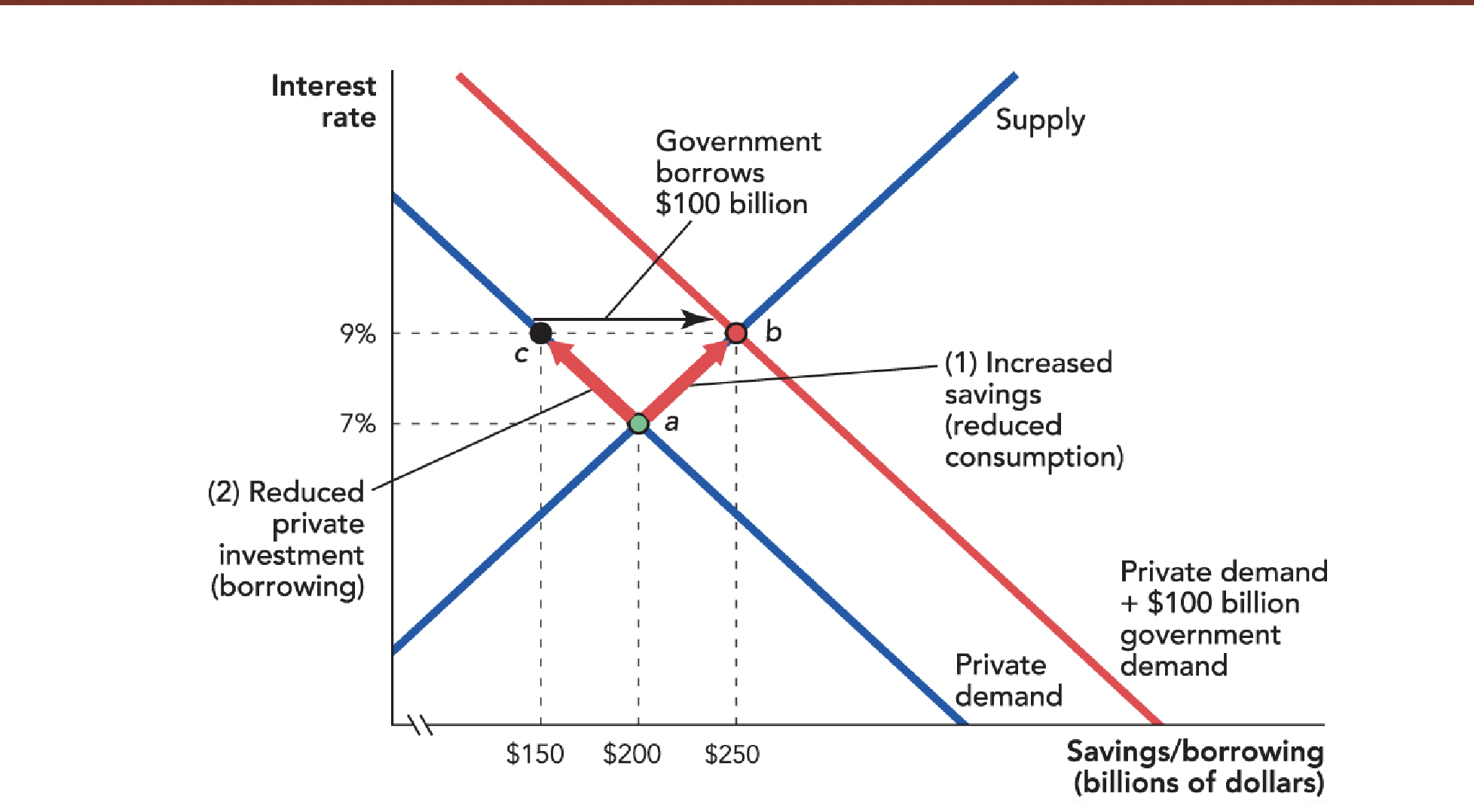
Why Should Fiscal Policy Work?

• If the resources used in new production would have otherwise

been unemployed, then every dollar spent will add one dollar to GDP.

• Increased spending by the previously unemployed workers could increase GDP by more than the initial amount.
• The additional increase in spending is due to the multiplier effect.

– The multiplier effect is the additional increase in spending caused

by the initial increase in government spending.

• Fiscal policy can work because when resources are unemployed, the economy is operating inefficiently

Self-Check:

An increase in government spending that causes a decrease in private spending is called: crowding out

Which of the following is not fiscal policy: Managing the money supply (this is part of monetary policy)

Why Should Fiscal Policy Work?

• A decrease in consumer spending growth, c, is equivalent to a decrease in velocity, v
• AD shifts to the left.
• The economy moves from a long-run equilibrium at point a to a short-run equilibrium at point b.
• At point b, the economy is in a recession.
• Because consumers want to hold more money, inflation decreases.
• Because wages are sticky, real growth decreases

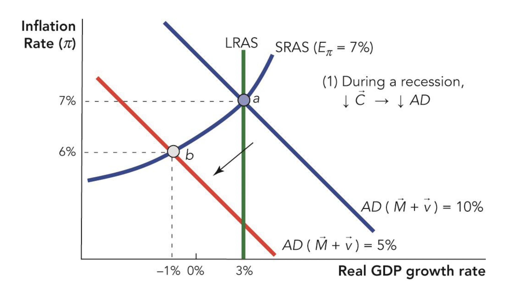
Fiscal Policy-The Best Case:

• If government does nothing, wages will adjust in the long run
• The economy will eventually return to its normal growth rate
• The government can offset decreasing C by increasing G
• The increase in government spending doesn’t have to be that large as the decrease in consumption because of the multiplier effect

The Size of the Multiplier:

• The debate over fiscal policy is about the balance of two opposing forces: crowding out versus the multiplier effect
• If additional government spending crowds out equivalent spending from the private sector, then the multiplier is zero.
• If no amount of private sector spending is crowded out, the multiplier is 1.
• If the increase in government spending causes additional private spending, the multiplier is greater than 1
• Fiscal policy is much more successful when the multiplier is big.
• The size of the multiplier is bigger when:

– There are lots of unemployed resources.

– The government can target spending on the unemployed.

– Tax cuts go to people who want to spend immediately.

– The government can tax savings.

– Government borrowing doesn’t crowd out private consumption or investment

April 19th Notes:

Government Borrowing and Crowding Out:

Higher interest rates leads to a reduced amount of private investment

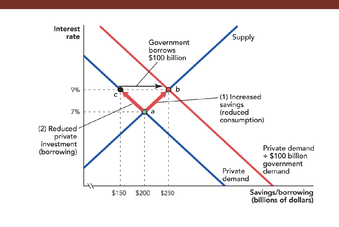
The Size of the Multiplier:

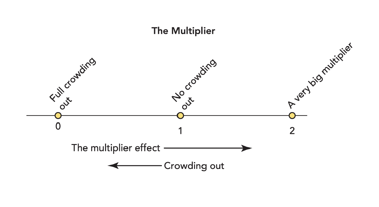
• Fiscal policy is much more successful when the multiplier is big
• The size of the multiplier is bigger when:

- There are lots of unemployed resources

- The government can target spending on the unemployed

- Tax cuts go to people who want to spend immediately

- The government can tax savings

- Government borrowing doesn’t crowd out private consumption or investment

Definition:

Ricardian equivalence:

• When people see that lower taxes today mean higher taxes in the future and so, instead of spending their tax cut, save it to pay future taxes. When Ricardian equivalence holds, a tax cut doesn’t increase aggregate demand even in the short run

Estimating the Multiplier:

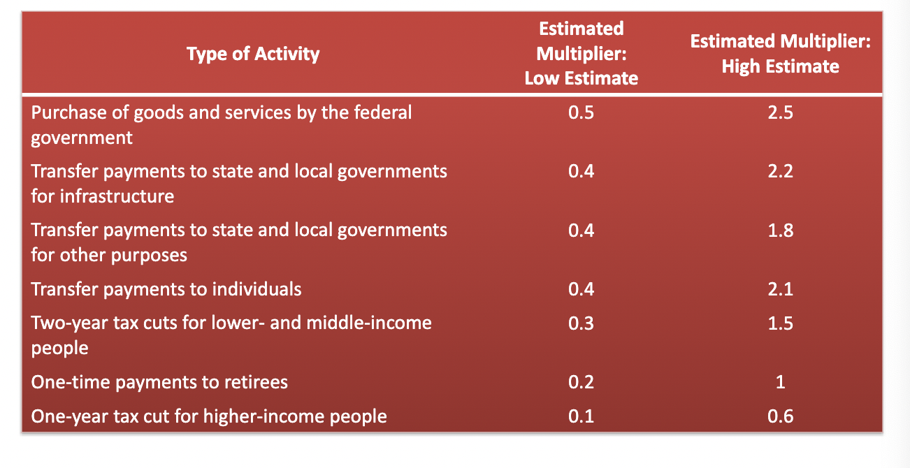
Limits to Fiscal Policy-Magnitude:

• Government spending doesn’t change very much from year to year in percentage terms
• Most of the federal budget is determined well in advance and is remarkably stable
• Any changes are not large enough in the short run to boost aggregate demand very much

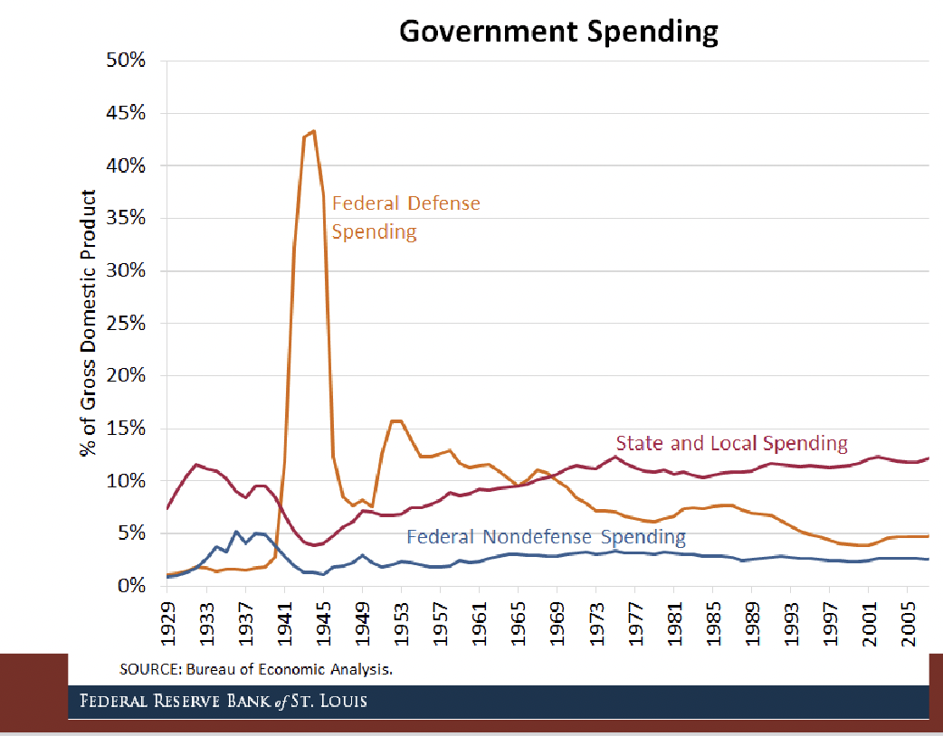
Limits to Fiscal Policy-Timing:

• Fiscal policy is subject to many lags:

1. Recognition lag: The problem must be recognized
2. Legislative lag: Congress must propose and pass a plan
3. Implementation lag: Bureaucracies must implement the plan
4. Effectiveness lag: The plan takes time to work
5. Evaluation and adjustment lag: Did the plan work? Have conditions changed?

• Tax cuts–the other major form of fiscal policy–also involve lags and uncertainties.
• Monetary policy is subject to lags as well, but these are generally much shorter than those for fiscal policy
• Fiscal policy is rarely adjusted in response to changes in economic conditions
• The only place where fiscal policy might have an advantage over monetary policy is through the effectiveness lag
• Exception: Automatic stabilizers are built right into the tax and transfer system

- Automatic stabilizers are changes in fiscal policy that stimulate AD in a recession without the need for explicit action by policymakers

• They take effect without significant lags

Automatic Stabilizers:

• Fiscal policy automatically changes to keep private spending higher during bad economic times
• When the economy is doing poorly:

- Income, capital gains, and profits are all down, so everyone pays lower taxes

- More people apply for welfare, food stamps, and unemployment insurance

• Consumption smoothing and credit also act as automatic stabilizers

The time it takes for fiscal policy to work is called the: effectiveness lag

Government Spending vs. Tax Cuts:

• The two types of fiscal policy differ politically and economically
• A tax cut or tax rebate puts more spending in the hands of the private sector
• An increase in government spending puts more spending in the hands of the government
• If we can find productive public investments such as improvements to schools, science funding, and infrastructure, then the case for public investment is strong

Balancing Fiscal Policy:

• Despite its limited magnitude and timing, some fiscal stimulus can make sense as part of the economy’s response to the business cycle
• Have to pay for this stimulus eventually

- Government surpluses balancing out government deficits will shrink AD–causing unemployment

- The resulting unemployment will be the smallest when the economy is booming–as will crowding out

- It makes sense for governments to pursue a counter-cyclical fiscal policy, which runs opposite or counter to the business cycle–spending more when the economy is in a recession, and spending less when the economy is booming.

Fiscal Policy and Real Shocks:

• When a real shock reduces the productivity of labor and capital, LRAS decreases
• An increase in government spending will increase aggregate demand
• However, due to the real shock, the economy is now less productive, so most of the increase will be felt as higher inflation rather than as real growth
• Fiscal policy is therefore not always an effective method of combating a recession

Fiscal Policy is Less Effective at Combating a Real Shock-

A real shock shifts the long-run aggregate supply curve (LRAS) to the left (step 1), moving the economy from point a to a recession at point b.

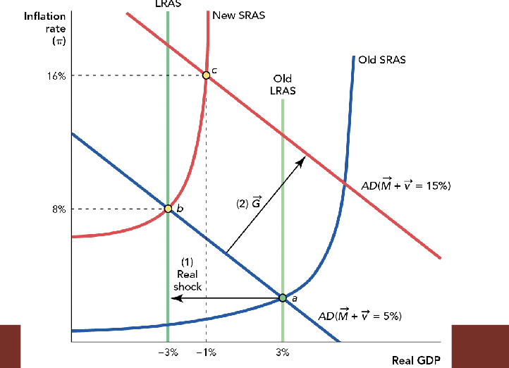
Covid and Fiscal Policy:

• The COVID-19 pandemic was a real shock because our abundance of caution made it more costly for people to work together.
• This shifted the LRAS supply curve to the left.
• Policymakers worried that getting people back to work could
• make the pandemic worse.
• Fiscal policy focused on temporarily protecting jobs and
• addressing the health costs of the pandemic.
• Overall, the U.S. federal government spent more than $5 trillion on COVID-19 relief.

Counter-Cyclical vs. “Common Sense” Fiscal Policy:

• Increased spending and tax cuts today tend to be followed by decreased spending or tax increases tomorrow.
• When spending falls and taxes rise, AD will fall—this is one reason why long-run or net multipliers are smaller than short-run multipliers.
• Spending more in bad times when the multiplier is big, and taxing more in good times when the multiplier is small, will lead to higher GDP overall.
• Again, this is the case for governments to pursue a counter-cyclical fiscal policy
• Ideal fiscal policy will increase AD by spending in bad times and reduce AD by taxing and paying off the bill in good times.
• Makes both the busts and booms smaller and the economy less volatile.
• Ideal fiscal policy is counter-cyclical because when the economy is down, the government should spend more, and when the economy is up, the government should

spend less.

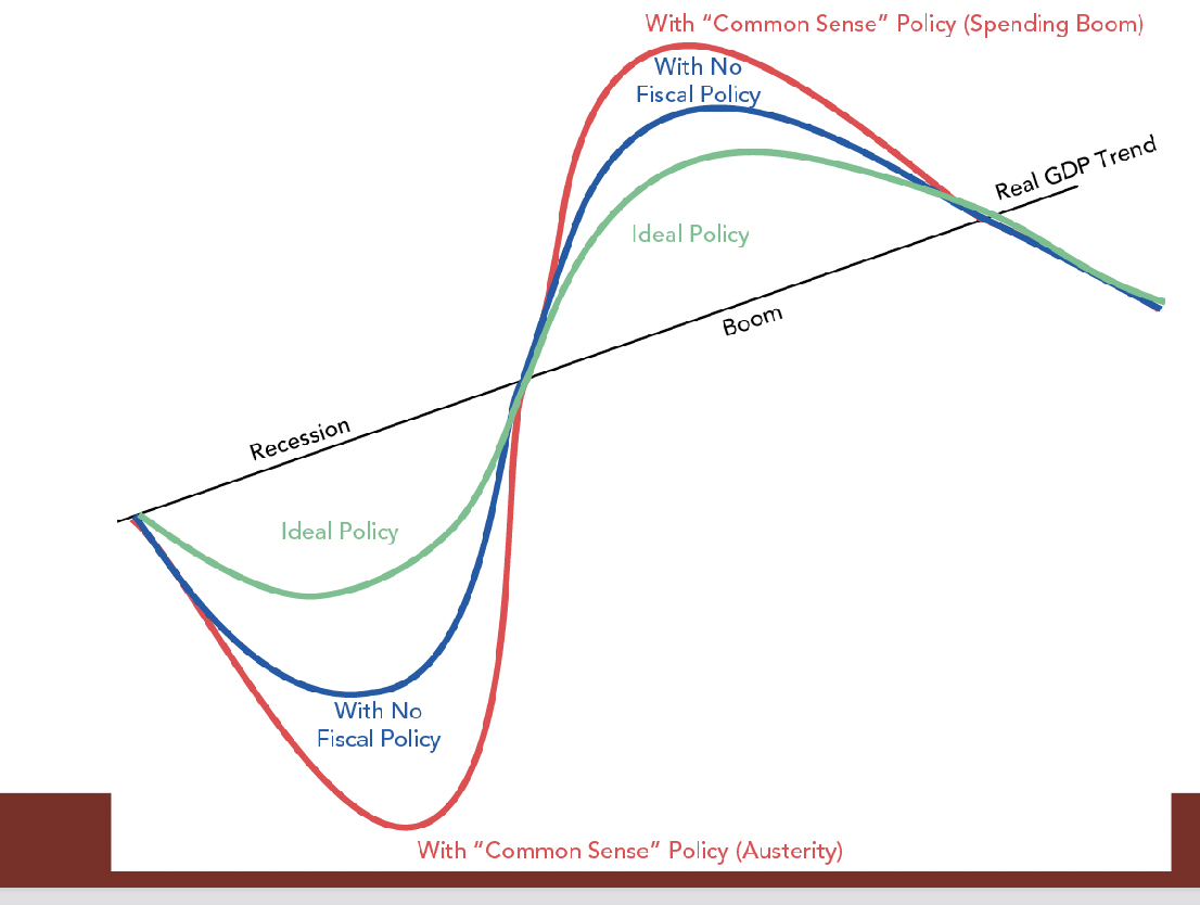
• Common sense fiscal policy also warns about having too much debt
• In extreme situations, debt can be such a problem that expansionary fiscal policy can reduce real growth

- Some countries are so heavily in debt that any more government borrowing runs the risk of total economic collapse

• In this setting, if the government increases spending, aggregate demand falls because uncertainty causes people to save or hoard their money in anticipation of hard times

When Fiscal Policy is a Good Idea:

The stimulus under President Barack Obama-

• A lot of the tax cuts were saved or used to pay off

debts, rather than spent.

• This boosted economic security for some people but

didn’t reemploy a lot of workers.

• The grants to the states prevented many state-

government layoffs, which was good for economic

Output.

Chapter 21 Notes:

• Public Choice: The study of political behavior using the tools of economics
• Behavioral symmetry: Self-interest is as important in politics as in economics
• Comparitive institutional analysis is all about analyzing the incentive issues associated with alternative institutional arrangements

Voters and the Incentive to be Ignorant:

• Studying politics doesn’t pay because the outcome of an election is mostly determined by what other people do, not by what you do
• Rationally ignorant: The incentives to be informed are low so people choose not to be informed
• The two largest sources of government spending are defense and Social Security
• Most Americans know “not much” or “nothing” about important pieces of legislation such as the USA Patriot Act.
• Most Americans cannot estimate the inflation rate or the unemployment rate to within five percentage points

Why Rational Ignorance Matters:

• If voters don’t know what the USA Patriot Act says or what the unemployment rate is, then it’s difficult to make informed choices
• Voters are supposed to be the drivers in a democracy, but if the drivers don’t know where they are of where they want to fo or how to get there, they are unlikely to ever arrive at a desirable destination
• Voters who are rationally ignorant will often make decisions on the basis of low-quality, unreliable, or potentially biased information
• Not everyone is rationally ignorant

Special Interests and the Incetive to be Informed:

Quota Example-

• Even if sugar consumers did know about the quota, they probably wouldn’t spend much time or effort to oppose it
• Sugar consumers won’t do much to oppose the quota, but U.S. sugar producers benefit enormously from quotas
• Sugar production is concentrated among a handful of producers. Each producer benefits from the quota by millions of dollars
• Sugar producers have more money at stake, which is a strong incentive to be rationally informed. For example, they know which politicians are running for election and donate accordingly.
• 13 of 21 senators on the Agricultural Committee received money from the American Crystal Sugar PAC. Many senators also received money from the American Sugar Cane League, the Florida Sugar Cane League, etc.

A Formula for Political Success-Diffuse Costs, Concentrate Benefits-

• The politics behind the sugar quota illustrate a formula for political success, diffuse costs and concentrate benefits
• The people who are harmed are rationally ignorant and have little incentive to oppose the policy, while the people who benefit are rationally informed and have strong incentives to support the policy. Therefore, we can see one reason why the self-interest of politicians doesn’t always align with the social interest
• The formula for political success works for many types of public policies, not just trade quotas and tariffs
• Agricultural subsidies and price supports fit the diffused costs and concentrated benefits story. The political power of farmers has increased as the share of farmers in the population has decreased. When farmers decline in population, the benefits of, for example, a price support become more concentrated on farmers and the costs become more diffused on nonfarmers
• The benefits of many government projects such as roads, bridges, dams, and parks are concentrated on local residents and producers, while the costs of these projects can be diffused over all federal taxpayers.
• Example: A ferry service runs to the island but some people in the town complain that it costs too much. If the town’s residents had to pay the $320 million cost of the bridge themselves

- As far as the residents of the town are concerned, the costs of the bridge are external costs

• The formula for political success works for tax credits and deductions, as well as for spending. Tax breaks for various manufacturing industries have long been common, the term manufacturing was significantly expanded so that oil and gas drilling as well as mining and timber could be included as manufacturing industries
• Every year, Congress inserts many thousands of special spending projects, exemptions, regulations, and tax breaks into major bills.
• When benefits are concentrated and costs are diffused, resources can be wasted on projects with low benefits and high costs
• Example: A special interest group representing 1% of society that proposes a simple policy that benefits the special interest by $100 and costs society $100. The policy benefits the special interest by $100 and it costs the special interest just $1. The special interest group will certainly lobby for a policy like this
• No society can get rich by passing policies with benefits that are less than costs
• Example: The fall of the Roman Empire was caused in part by bad political institutions. As the Roman Empire grew, courting politicians in Rome became a more secure path to riches than starting a new business

Another Formula-Concentrated Costs, Diffuse Benefits:

• Policies with concentrated benefits and diffuse costs can win in a democratic process even when the benefits are less than the costs
• When costs are concentrated and benefits are diffused another government failure can happen–policies with concentrated costs and diffuse benefits can lose in a democratic system even when the benefits are more than the costs
• Many cities make it costly and dificult to build new housing. In a typical process, even when land is zoned for construction, a builder must also get approval from a neighborhood review board which holds hearings
• The costs of a project, whether real or imagined, are concentrated on a small number of people who are likely to be vocal about their opposition. The benefits are diffuse
• The developer will benefit and will speak in favor, but the future residents are probably unknown, even to themselves
• Diffuse beneficiaries are more likely to vote about general rules than they are to attend and speak at a review board about a specific proposal

Voter Myopia and Political Business Cycles:

• Rational ignorance and voter myopia can encourage politicians to boost the economy before an election to increase their chances of reelection
• Personalities and leadership loom large and are reckoned to swing voters one way or another
• Economists and political scientists have been surprised to discover that a simpler logic underlies this apparent chaos of seemingly unique and momentous events
• Voters are so responsive to economic conditions that the winner of a presidential election can be predicted with considerable accuracy, even if one knows nothing about the personalities, issues, or events that seem to matter so much
• For each presidential election since 1948, the share of the two-party vote won by the party of the incumbent

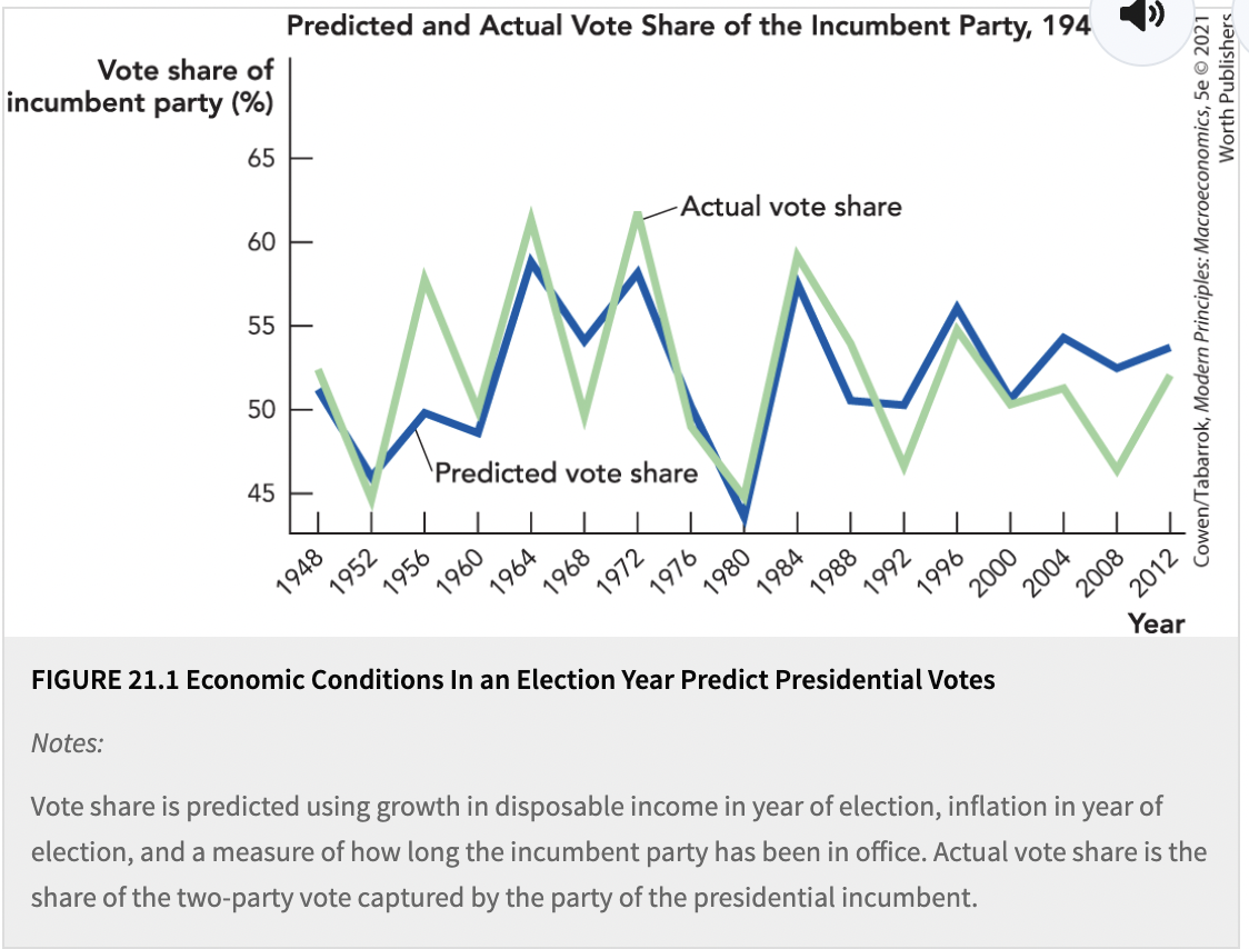
• The incumbent party wins elections when personal disposable income is growing, when the inflation rate in the election year is low, and when the incumbent party has not been in power for too many terms in a row
• The inflation rate is the general increase in prices. Voters seem to get tired or disillusioned with a party the longer it has been in power, so there is a natural tendency for the presidency to switch parties even if all remains the same
• Voters are myopic–they don’t look at economic conditions over a president’s entire term
• Politicians who want to be reelected, therefore, are wise to do whatever they can to increase personal disposable income and reduce inflation in the year of an election even if this means decreases in income and increases in inflation at other times
• Inflation also follows a cyclical pattern, but since voters dislike inflation, it tends to decrease in the year of an election and increase after the election
• Mayors and governors try to increase the number of police on the streets in an election year, so that crime will fall and people will feel safer
• Presidents don’t always succeed in increasing income during an election year

Two Cheers for Democracy:

• When a policy is specializwd in its impact, difficult to understand, and affects a small part of the economy, it is likely that special interests get their way
• When a policy is highly visible, appears often in the news and on social media, and has a major effect on the lives of millions of Americans, the voters are likely to have an opinion.

The Median Voter Theorem:

• Example: There are five voters, each who has an opinion about the ideal amount of spending on Social Securiy. Each voter’s ideal policy is along a line from least to most spending.

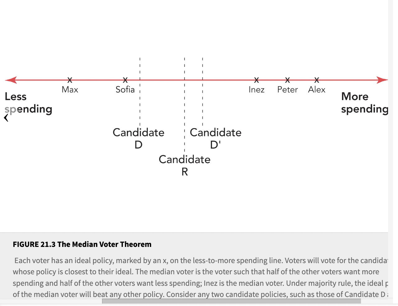
• The median voter theorem:Says that when voters cote for the policy that is closest to their ideal point on a line, then the ideal point of teh median voter will beat any other policy in a majority rule election
• Of the two policies being offered, the closest to that of the median voter’s ideal policy won the election
• The median voter theorem can be interpreted as the standard political spectrum of left to right
• The median voter theorem tells us that in a democracy, what counts are noses–the number of voters–and not their positions per se
• The most important assumption for the median voter theorem is that voters will vote for the policy that is closest to their ideal point
• Example: If no candidate offers a policy close to Max’s ideal point, he may refuse to vote for anyone, not even the candidate whose policy is slightly closer to his ideal
• A candidate who moves too far away from the voters on her wing may lose votes even if her position moves closer to that of the median voter
• As a result, this type of voter behavior means that candidates do not necessarily converge on the ideal point of the median voter
• The U.S. Constitution requires that new legislation must pass two houses of Congress and evade the president’s veto, which is more difficult than passing a simple majority rule vote

Democracy and Nondemocracy:

• Democracies tend to be the wealthiest countries, and despite the power of special interests, they also tend to be the countries with the best record of supporting markets, property rights, the rule of law, fair government, and other institutions that support economic growth
• There is an association between democracy and the standard of living because greater wealth creates a greater demand for democracy
• In many quasi democracies and in nondemocracies, the public is not well informed because the media are controlled or censored by the government
• Example: In Africa most countries have traditionally banned private television stations. Most African governments control the largest newspapers in the country
• Control of the media enables special interests to control the government for their own ends
• Citizens in democracies may be rationally ignorant, but on the whole they are much better informed about their governments than citizens in quasi democracies and nondemocracies
• In a democracy, citizens can use their knowledge to influence public policy at low cost by voting. In non democracies, knowledge is not enough because intimidation and government violence create steep barriers to political participation
• The importance of knowledge and the power to vote for bringing about better outcomes is illustrated by the shocking history of mass starvation

Democracy and Famine:

• Many of the famines in recent world history have been intentional.
• Stalin collectivized Ukranian farms and expropriated the land of the kulaks, turning them out of their homes and sending hundreds of thousands to gulag prisons in Siberia.
• Agricultural productivity in Ukraine plummeted under forced collectivization and people began to starve. Stalin continued to ship found out of Ukraine
• Mass starvation occurred not because of a lack of food per se, but because a poor group of laborers lacked both economic and political power
• Amartya Sen argued that “no famine has taken place in the history of the world in a functioning democracy”
• Economists Timothy Besley and Robin Burgess have tested Sen’s theory of democracy, newspapers, and famine relief in India. They as whether state governments are more responsive to food crises when there is more political competition and more newspapers. Government is more responsive to a crisis in food availability when newspaper circulation is higher
• It’s only when democratic politicians face the right incentives due to competitive elections and good information that their incentives become more aligned with the social good

Democracy and Growth:

• One reason for the good record of democracies on economic growth may be that the only way the public as a whole can become rich is by supporting efficient policies that generate economic growth
• Nondemocratic elites may not want to support mass education. The elites will often want to keep the masses weak and uninformed, neither of which is good for economic growth or, for that matter, preventing starvation
• The larger the group, the greater the group’s incentives to take into account the social costs of inefficient policies
• The greater the share of the population that is brought into power, the more likely that policies will offer something for virtually everybody, and not just riches for a small elite

Takeaways:

• Rational ignorance means that special interests can dominate parts of the political process. By concentrating benefits and diffusing costs, politicians can often build politcal support for themselves even when their policies generate more costs than benefits
• Incumbent politicians can use their control of the government to increase the probability that they will be reelected
• When markets fail to align self-interest with the social interest, we get market failure. No institutions are perfect and trade-offs are everywhere–this is a key lesson when thinking about markets and government
• It’s hard for politicians in a democracy to ignore the major interest of voters

April 22nd Notes:

Political economy, or public choice, uses the tools of economics to study political behavior

Rational Ignorance:

• Most Americans know very little about political matters

- When Americans were asked the two largest sources of government spending out of six, 41% named the smallest: foreign aid

- Most Americans say they know “not much” or “nothing” about important legislation such as the USA Patriot Act

- Most cannot estimate unemployment or inflation to within five percentage points

• These are examples of rational ignorance, where the benefits of being informed are less than the costs of becoming informed
• The incentives to be well informed about politics are low. Doesn’t offer much return, and studying politics doesn’t pay because elections are mostly determined by what other people do, not by what you do

Why Rational Ignorance Matters:

1. If voters don’t know the facts, then it’s difficult to make informed choices
2. Rationally ignorant voters often make decisions on the basis of low-quality, unreliable, or potentially biased information
3. Not everyone is rationally ignorant

The Incentive to be Informed:

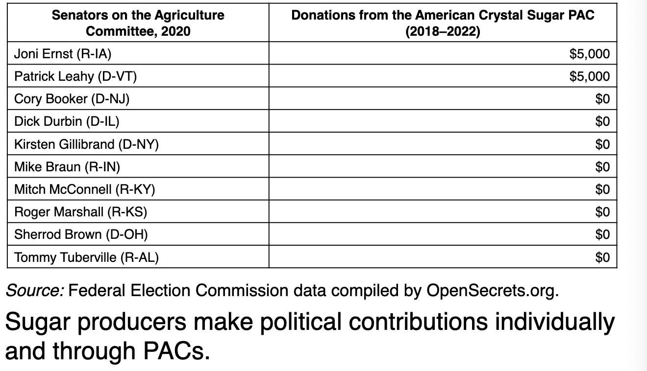
Quotas:

• While tariffs tax imports, quotas directly restrict the quantity of goods that can be imported
• Like tariffs, they raise the price of imported goods above the world price
• This shrinks consumer surplus
• But increases producer surplus

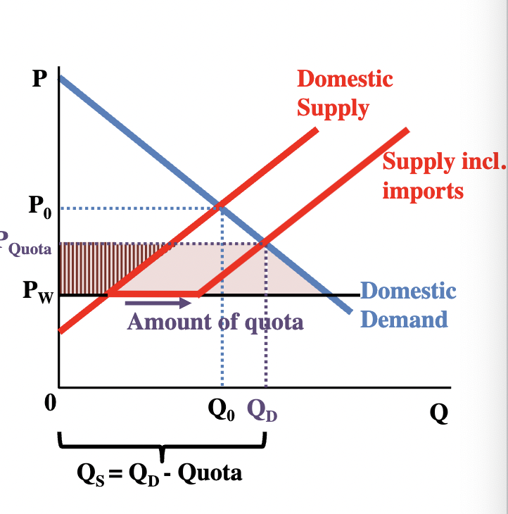
The Incentive to be Informed Example:

• Sugar producers have anb incentive to ve rationally informed because they have a lot of money at stake and each producer benefits from the quota by millions of dollars
• Self-Check: Who has the greatest incentive to be informed about an import quota on clothing? Domestic producers

Diffiuse Costs, Concentrate Benefits:

• The self-interest of politicians doesn’t always align with the social interest
• One formula for political success is to diffuse costs and concentrate benefits

- The people who are harmed are rationally ignorant and have little incentive to oppose the policy

- The people who benefit are rationally informed and have strong incentives to support the policy

• This formula for political success works for many types of public policies-

- Trade quotas and tariffs

- Agricultural subsidies and price supports

- Government projects such as roads, bridges, dams, and parks

- Tax credits and deductions

• When benefits are concentrated and costs are diffuse, resources can be waste don projects with low benefits and high costs

Voter Myopia and Political Business Cycles:

• Over the past 100 years, Americans have voted for the party of the incumbent when the economy is doing well and against the incumbent when the economy is doing poorly
• More specifically, the incumbent party wins when:

- Personal disposable income is growing.

- The inflation rate is low, and

- The incumbent party has not been in power for too many terms in a row.

• Voters don’t look at economic conditions over a president’s entire term
• They focus on economic conditions in the year of an election
• Politicians who want to be reelected do whatever they can to increase personal disposable income and reduce inflation in the year of an election

Voter Myopia and Political Business Cycles:

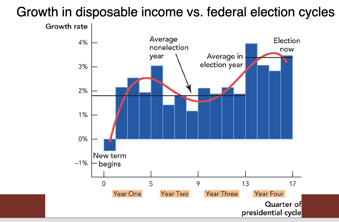
Two Cheers for Democracy:

• Lobbies and special interests are likely to get their way when a policy:

- Is specialized in its impact

- Is difficult to understand

- Affects a small part of the economy

• Voters are likely to have opinions when a policy:

- Is highly visible

- Appears often in the media

- Has a major effect on the lives of millions of Americans

The Median Voter Theorem:

• Definition: When voters vote for the policy that is closest to their ideal point on a line, then the ideal point of the median voter will beat any other policy in a majority-rule election

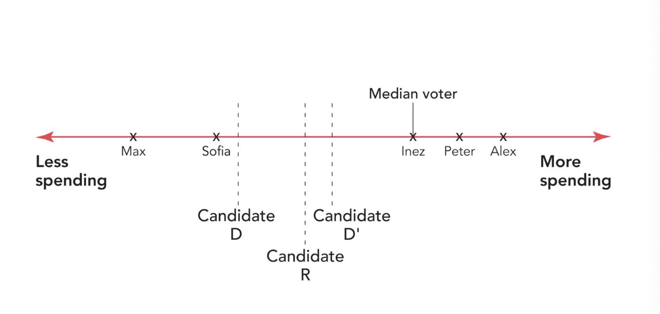
• According to the median voter theorem, the median voter rules
• If the median voter doesn’t change, then neither does policy
• Under the conditions of the theorem, democracy does not seek out consensus or compromise or a policy that maximizes voter preferences
• Instead, it seeks out a policy that cannot be beaten in a majority-rule election
• The theorem does not apply if:

- Voters don’t vote for the policy that is closest to their ideal point

- There is more than one major dimension over which voting takes place

• Sometimes a winning policy doesn’t exist
• The theorem indicates that politicians have substantial incentives to listen to voters on issues that the voters care about

Democracy and Nondemocracy:

• The countries that are most democratic are among the wealthiest countries and have the most economic freedom
• There is a strong correlation between democracy and a high standard of living
• This is partially because greater wealth creates a greater demand for democracy

Economic Freedom, Democracy, and Living Standards:

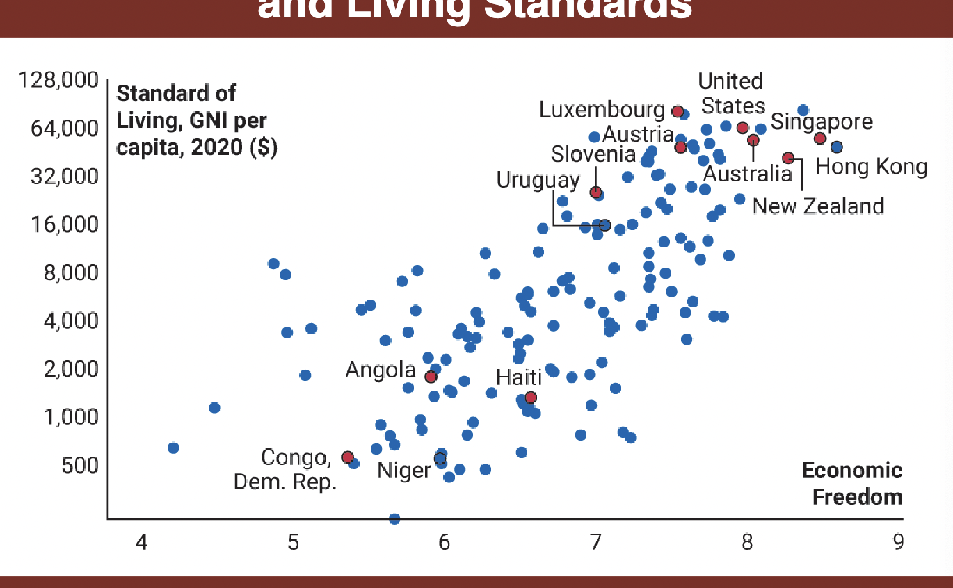
Democracy and Famine:

• Many famines have been intentional
• When Stalin came to power in 1924, he saw wealthy independent farmers as a threat
• He collectivized the farms, expropriated the land, and sent hundreds of thousands of people to prisons
• Agricultural productivity in Ukraine plummeted, but food was still shipped out of the country and millions of Ukranians died
• The famine is less likely to have happened in a democracy
• Nobel Prize winner Amartya Sen has said, “No famine has taken place in the history of the world in a functioning democracy.”
• Economists Timothy Besley and Robin Burgess have tested Sen’s theory
• They found that:

- Greater political competition is associated with higher levels of public food distribution

- Government is more responsive to a food crisis when newspaper circulation is higher

Democracy and Growth:

• Democracies have a good record of supporting institutions that promote economic growth:

- Markets

- Property rights

- The rule of law

- Fair government

• The only way the public can become rich is through policies that generate economic growth
• Nondemocratic elites become rich by dividing the pie in their favor even if it means a smaller pie

Takeaways:

• Voters in a democracy often have little incentive to be informed about political matters
• Rational ignorance means that special interests can dominate parts of the political process
• Politicians can build support by concentrating benefits and diffusing costs
• Voters focus on current economic conditions
• Politicians typically increase spending before an election
• The record of democracies on some of the big issues is quite good
• Politicians in a democracy can’t ignore the major interests of voters
• If things do go wrong, voters in a democracy can vote the politicians out