Health State Valuation and Preference-Based Measures (QALYs, DALYs, MAUIs)
Session Aims
Introduce approaches for measuring health in evaluations.
Define the Quality-Adjusted Life Year (QALY) and common derivation methods.
Present generic preference-based measures (Multi-Attribute Utility Instruments, MAUIs).
Highlight limitations of QALYs and measurement instruments.
Learning Objectives
Understand the assumptions and calculation of QALYs.
Distinguish QALYs from Disability-Adjusted Life Years (DALYs).
Explain preference-elicitation techniques: TTO, SG, VAS, DCE, BWS.
Identify available generic MAUIs, their development, and scoring.
Reflect on limitations and inter-instrument differences.
Economic Evaluation: Context
Requires measurement of both costs and benefits.
Benefit measurement varies by evaluation type; cost-utility analysis uses utility instruments to generate QALYs.
Recall 8 stages: Clarify question → Identify consequences → Quantify → Value → Analyse → Interpret → Decision-maker use.
Defining Health & HRQoL
WHO (1948): “A state of complete physical, mental and social well-being…”.
Distinction between health vs. broader quality-of-life aspects.
Health-related quality of life (HRQoL): QoL domains affected by health/treatment.
Measures differ in content; some labelled HRQoL but focus only on symptoms.
Measuring Health
Discrepancies often observed between clinician vs. patient reports.
Preference for self-report (e.g., SF-36); item generation increasingly patient-led.
Identifying Outcomes
Surrogate/Intermediate outcomes (e.g., HbA1c, viral load, vaccine uptake).
Final outcomes: mortality & morbidity (LYs, QALYs gained, DALYs avoided).
Example Instrument: SF-36
8 domains, 36 items; each domain scored 0\text{–}100.
Domains, items, ranges: Physical Functioning (10, 10–30) … General Health (5, 5–25).
Two summary scores: Physical (PCS) & Mental (MCS).
Equal weighting assumption problematic for economic evaluation (e.g., vigorous vs. moderate activity limitation treated equally).
Trial example: mixed domain changes—unclear overall benefit without preference weighting.
Quality-Adjusted Life Years (QALYs)
Combine survival (quantity) and HRQoL (quality) into “years in full health”.
Anchors: 1=\text{full health}, 0=\text{death}, <0=\text{worse than death}.
Calculation: \text{QALY}=\sum{t} Qt\times T_t.
Example: 20 years on dialysis, weight 0.8 \Rightarrow 20\times0.8=16\text{ QALYs}.
10 years at uitility weight 0.6 ⇒ 6\text{ QALYs}.
Graphical interpretation: area under quality–time curve.
Disability-Adjusted Life Years (DALYs)
\text{DALY}=\text{YLL}+\text{YLD}.
One DALY = 1 year of full-health lost; weights: perfect health 0, death 1.
Goal: minimise DALYs (or maximise DALYs averted).
Broad relation: \text{DALYs averted} \approx \text{QALYs gained}.
Expected QALYs Under Uncertainty
Treatments have probabilistic future utilities.
Example table (1-year horizon):
Treatment A: P(\text{cure})=0.70, P(\text{no change})=0.20, P(\text{adverse})=0.10.
Combine with utilities (1, 0.8, 0.3) to compute expected QALY.
Core Assumptions Behind QALYs
Independence of quality (Q) and time (T): value unaffected by when/how long.
5\text{ yrs}@0.9 = 6\text{ yrs}@0.75 = 45\text{ yrs}@0.1.
Linearity in probability (risk neutrality).
0.1\times10\text{ QALYs}+0.9\times0=1\text{ QALY}.
Additive separability over time (no state interaction effects).
3\text{ yrs}@0.2 + 5\text{ yrs}@0.8 = 5\text{ yrs}@0.8 + 3\text{ yrs}@0.2.
Preference-Elicitation Techniques
Time Trade-Off (TTO)
Standard Gamble (SG)
Visual Analogue Scale (VAS)
Ranking
Discrete Choice Experiment (DCE)
Best-Worst Scaling (BWS)
Person Trade-Off (not covered)
Time Trade-Off (TTO)
Sacrifice length for quality: choose between
t years in state i then death.
x<t years in full health then death.
Indifference ⇒ utility h_i = x/t.
Example: indifference at x=4, t=10 \Rightarrow h_i=0.4.
Variants: duration (10 yrs vs. life expectancy), administration mode, titration method, visual aids, context effects, response variable.
Advantages: choice-based, explicit Q–T trade-off, easier than SG probabilities.
Disadvantages: assumes constant proportional trade-off, ignores time preference, difficulty valuing ‘worse-than-dead’, comprehension issues.
Standard Gamble (SG)
Based on Expected Utility Theory (EUT).
Choice between certain state h_i and gamble: probability p of full health, 1-p of death.
Indifference ⇒ h_i = p.
Willingness to accept 10% death risk ⇒ h_i=0.9.
States worse than dead: swap positions; utility h_i= -p/(1-p) (bounded to -1 in practice).
Advantages: rooted in EUT, incorporates uncertainty, choice-based.
Disadvantages: probability comprehension, risk attitudes & loss aversion contaminate values, death framing concerns.
Visual Analogue Scale (VAS)
Rating thermometer 0-100 anchored at “worst/best imaginable health”.
For QALYs must anchor to death (0) and full health (100); recalibrate if necessary.
Calculation example: health state at 80, death at 20 ⇒ \frac{80-20}{100-20}=0.75.
Advantages: simple, cheap, high response.
Disadvantages: no sacrifice notion, end-aversion, spreading & context biases, yields ordinal data; mapping to TTO/SG possible but debated.
Discrete Choice Experiment (DCE) & Best-Worst Scaling (BWS)
DCE: respondents choose preferred state from pairs; modelled via Random Utility Theory (logit/probit), producing marginal utilities.
BWS: select best & worst attribute within a profile; extension of DCE.
Anchoring to 0–1 scale options: worst-state =0, hybrid with TTO/SG, include ‘dead’, mapping, logistic transformation with duration attribute.
DCE with duration overcomes ‘dead’ issue; closer to TTO concept.
Pros: potentially less cognitively demanding, online feasible.
Cons: no explicit sacrifice, possible heuristic use, modelling complexity, large samples.
Comparison of Valuation Methods
Criterion | VAS | TTO | SG | DCE |
|---|---|---|---|---|
Choice-based | ✗ | ✔ | ✔ | ✔ (if duration) |
Cardinal scale | ? | ✔ | ✔ | ✔ (some models) |
Economic theory | ✗ | ✗ | ✔ (EUT) | ✔ (RUT) |
Includes uncertainty | ✗ | ✗ | ✔ | ✗ |
Ease/Cost | High | Medium | Low | High (online=M) |
Typical pattern: \text{VAS}<\text{TTO}<\text{SG} values.
Choosing a Technique
VAS often ruled out for utility generation.
SG & TTO historically dominant but interview-intensive.
Ordinal methods (DCE/BWS) gaining popularity; cost & practicality advantages.
Multi-Attribute Utility Instruments (MAUIs)
Provide off-the-shelf scorings; two components:
Classifier (health description).
Tariff (pre-scored utilities from general-population valuations).
Advantages: cheap, comparable across studies, accepted by NICE & others.
Disadvantages: may lack sensitivity/relevance; differing domains, levels, valuation methods cause divergent utilities.
Common Generic MAUIs
EQ-5D-3L / EQ-5D-5L
SF-6D (from SF-36)
Health Utility Index (HUI 1-3)
AQoL-8D
QWB, PROMIS-29, 15D (Scandinavia)
EQ-5D Structure
5 dimensions: Mobility, Self-care, Usual Activities, Pain/Discomfort, Anxiety/Depression.
3L: 3 severity levels ⇒ 3^5=243 states.
5L: 5 levels ⇒ 5^5=3125 states.
EQ-5D Valuation Example (UK 3L tariff)
Regression on 3,395 general-population TTO interviews.
Utility for state 11223:
Constants & coefficients: -0.081, -0.036, -0.123, -0.236, -0.269 (N3 interaction).
U=1-0.081-0.036-0.123-0.236-0.269=0.255.
Other Instruments: Key Facts
Instrument | Valuation | Extrapolation | Sample |
|---|---|---|---|
EQ-5D-3L | TTO+VAS | Regression | GP (many countries) |
EQ-5D-5L | TTO+DCE | Regression | GP (growing) |
SF-6D | SG | Regression | GP (UK, Japan…) |
HUI3 | VAS→SG | MAUT | GP (Canada, France) |
AQoL-8D | VAS→TTO | MAUT | GP & patients (Australia, etc.) |
Differences Between Instruments
Coverage: e.g., vision in HUI, not EQ-5D.
Severity range (floor/ceiling): SF-6D narrow range at worst health.
Sensitivity: number of levels (EQ-5D-3L coarse at top end).
Scaling: divergent bottom values; not perfectly comparable.
Child-Specific Utilities
CHU9D, HUI2, EQ-5D-Y (Australian 3L value set 2025).
Adjusted descriptors, age targets, valuation challenges.
Whose Values? Public vs. Patients vs. Experts
NICE, ICER, WHO favour general-population values (taxpayer perspective, veil of ignorance).
Patients: firsthand experience but potential adaptation/response-shift; sometimes unable (children, severely ill).
Empirical finding: Public values ↓ for physical states, ↑ for mental health compared with patients.
Explanations: different reference frames, adaptation, focusing illusion.
Instrument Choice Considerations
Suitability: domains, sensitivity, target population, intervention effects.
Practicalities: length, cognitive burden, licensing cost, administration mode.
Cross-cultural response variation observed (e.g., Asians report fewer problems).
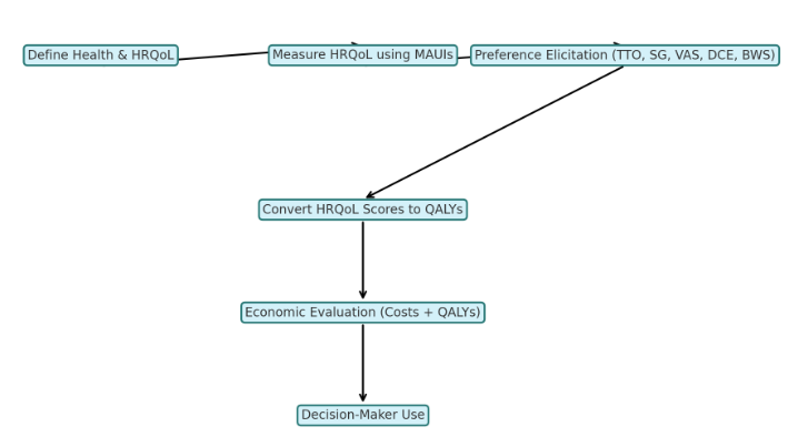
Health State Measurement & Valuation Pathways
Non-preference instruments (e.g., SF-36) → map to utilities.
Direct elicitation (TTO/SG/DCE) → utility scores.
MAUIs (generic or condition-specific) directly yield utilities.
Summary
QALYs enable comparison across diseases/interventions by combining quantity and quality of life.
Utility estimates derived via direct elicitation or pre-scored MAUIs; each method/instrument has strengths, weaknesses, and assumptions.
Core QALY assumptions (independence, linearity, additivity) are pragmatic simplifications enabling practical modelling.
Selection of valuation technique and instrument should consider theoretical soundness, cognitive burden, sensitivity, cost, and decision-maker guidelines.