6.1 Discrete and Continuous Random Variables

Discrete Random Variables:

• Random Variable represents the possible outcomes of a random process

  • AKA Random Result

  • Ex: X = number of heads in three tosses

  • Always a capital, italic letter (like X or Y)

• The Probability distribution describes the likelihood of various outcomes (random variables), along with their probabilities.

  • Two Requirements:

  • Every probability p_i is a number between 0 and 1, inclusive.

  • The sum of the probabilities is 1: p₁ + p₂ + p₃ + . . . = 1.

• A discrete random variable has specific, separate, and often whole number values / outcomes

  • Like (1, 2, 3, etc.) on a die

  • Discrete usually counts

    • Digital input in CS

    • Ex: like number of siblings

• For random variabilities (probability in general), use mean instead of median

  • Mean is represented as mu or μ (usually with a subscript of the random variable)

  • Ex: Random Variable X, mean = μ_x

Analyzing Discrete Random Variables

• In a Histogram, analyze: shape, center, and variability

• Shape Options: Skewed Left/Right & Symmetric

  • Symmetric can be bimodal or unimodal

  • Normal curve is always symmetric unimodal

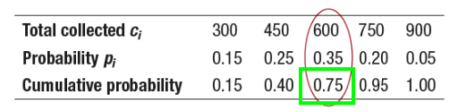
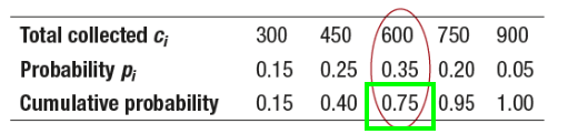
  • Ex: The graph is roughly symmetric and has a single peak at $600

• Mean (expected value) of a discrete random variable is the average value in a random process

  • Important Part: Expected Value takes frequency into consideration

    • Don’t take an average of Random Variables (X), since each random variables have different weights / frequencies than others.

  • Formula: μ_x = E(X) = x₁p₁ + x₂p₂ + x₃p₃ + … = ∑ x_{i *} p_i

  • Ti-Nispire Usage:

    • Spreadsheet → Enter Data into 2 Columns

    • Menu → Statics → Stat Calculations → Two-Variable Statistics

    • Answer is value of ∑ xy

• Median is when the cumulative probability equals or exceeds 0.5

  • 

• Standard Deviation aka σ (omega)

  • Ti-Nispire Usage:

    • Spreadsheet → Enter Data into 2 Columns

    • Menu → Statics → Stat Calculations → Two-Variable Statistics

    • Answer is value of σx

  • Variance is (Standard Deviation)²

Discrete Random Variable Example Problem:

Continuous Random Variables:

• A Continuous Random Variable takes any value in an interval on the number line (range)

  • Continuous usually measures

    • Analog input in Computer Science

    • Ex: height of a student or time to run a mile

• To find its probabilities, use a Density Curve

  • • 1/9 × 9 = 1 (Probability always adds to 1)

  • 

Continuous Example Problem:

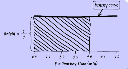
Question: Would it be faster to take the train or walk? Walking takes 4 mins. What is the probability that Selena's train journey time to work is shorter than her walking time, given that her train journey time (Y) follows a uniform distribution from 2 to 5 minutes?

Solution:

1. Identify Continuous vs Discrete. This situation involves time (measured), so continuous .

2. Form the density curve: 5.0 - 2.0 = 3 → 3 × 1/3 = 1 (Probability adds to 1)

   1. 

3. Calculate Shaded Area: base × height = (4.0 - 2.0 ) × 1/3 = 2/3

4. → P(Y < 4) = 2/3 = 0.667

5. Sentence: There is a 66.7% chance that it will be quicker for Selena to take the train to work on a randomly selected day.

Question: The heights of young women can be modeled by a Normal distribution with mean µ = 64 inches and standard deviation σ = 2.7 inches. Suppose we choose a young woman at random and let Y = her height (in inches). Find P(68 ≤ Y ≤ 70). Interpret this value.

TODO: Insert Normal Curve Drawing

Answer: normalCdf(lower: 68, upper: 70, mean: 64, SD: 2.7) = 0.051

6.2 Transforming and Combining Random Variables

• Adding the same positive number a to (subtracting a from) each value of a random variable:

  • Adds a to (subtracts a from) measures of center and location (mean, median, quartiles, percentiles).

    • Mean of Sum/Difference of Random Variables: μ_s = μ_x+-y = μ_x +- μ_Y

  • Does not change measures of variability (range, IQR, standard deviation).

    • Variance adds (and subtracts), standard deviations do not add / subtract.

  • Does not change the shape of the probability distribution.

• Multiplying (or dividing) each value of a random variable by the same positive number b:

  • Multiplies (divides) measures of center and location (mean, median, quartiles, percentiles) by b.

  • Multiplies (divides) measures of variability (range, IQR, standard deviation) by b.

  • Does not change the shape of the distribution.

• Linear Transformation: If Y = a+ bX is a linear transformation of the random variable X,

  • The distribution of Y has same shape as the probability distribution of X if b > 0

  • μ_Y = a+ bμ_X

  • σ_Y = |b|σ_X (because b could be a negative number)

Adding / Subtracting Example Problem:

Question: Score X of a randomly selected student on a test worth 50 points can be modeled by a Normal distribution with mean 35 and standard deviation 5. Professor decides to add 5 points to
each student’s score. Let Y be the scaled test score of the randomly selected student. Describe the shape, center, and variability of the probability distribution of Y.

Answer:

• Shape: Approximately Normal

• Center: µ_Y = µ_X + 5 = 35 + 5 = 40

• Variability: σ_Y = σ_X = 5

Multiplying / Dividing Example Problem:

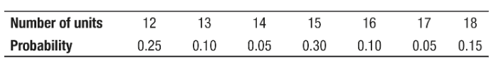
Question: Student is full-time if taking 12 and 18 units. The number of units X that a randomly selected El Dorado Community College full-time student is taking (see histogram). Mean is µX = 14.65 and the standard deviation is σX = 2.056. Tuition is $50 per unit. If T = tuition charge for a
randomly selected full-time student, T = 50X.

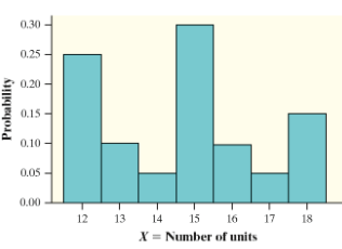
Answer:

• Shape: Same shape as the probability distribution of X, roughly symmetric with three peaks.

• Center: µ_T = 50µ_X = 50(14.65) = $732.50

• Variability: σ_T = 50σ_X = 50(2.056) = $102.80

Linear Transformation Example Problem:

Question: Let X = the number of passengers on a randomly selected trip at Pete’s Jeep Tours. Let Y = the number of passengers on a randomly selected trip at Erin’s Adventures. What is the sum S = X + Y of the number of passengers Pete and Erin will have on their tours on a randomly selected day?

Answer:

6.3 Binomial and Geometric:

Binomial Random Variables

• Binomial Setting is when n independent trials are committed with a sauce chance of an outcome (aka success) occurs. Test using BINS

  • Binary? Possible outcomes should be “success” or “failure”

  • Independent? Trials must be independent. Knowing the outcome of one trial can’t determine another trial.

  • Number? The number of trials must be fixed in advance

  • Same Probability? Probability must be of success p on each trial.

• Binomial Random Variable is the count of successes X in a binomial setting (literally a discrete variable)

• Binomial Distribution is the probability distribution of X.

  • n trials and probability p of success on each trial.

• Binomial Coefficient arranges k successes with n trials.

  • (n/k) = (n! / ( k! * (n-k)! ))

• Binomial Probability Formula uses the Binomial Coefficient

  • Actual formula on equation sheet - P(X = x) = (n / x)…

  • binompdf (n,p,k) computes P(X = k)

  • binomcdf (n,p,k) computes P(X ≤ k)

• Steps to find Binomial Probabilities:

  • State the distribution and the values of interest. Specify a binomial distribution with the number of trials n, success probability p, and the values of the variable clearly identified.

  • Perform the calculations, show calculator steps (or formula)

  • Be sure to answer the question

• Center & Variability (Only for Binomial Distributions):

  • Mean - μ_x = E(X) = np

  • SD: σ_X = root( np * (1 - p) )

• 10% Rule: A distribution will be approximately binomial when the sample size n is less than 10% of the population (Overrides BINS)

  • # of trials < 0.10 * population

  • Ex: A starburst bag comes with 200 candies. 25% chance one candy is red. This is not independent, and fails BINS. But since there are more than 200 starbursts in the world, the 10% rule applies. This distribution is approximately binomial.

• Large Counts Condition: probability distribution of X is approximately normal if:

  • np ≧ 10 AND n( 1-p ) ≧ 10

  • AKA: Expected Numbers (mean) of successes and failures is at least 10

Geometric Random Variables

• Geometric setting exists when the number of trials is unknown. Independent trials are performed until one success is made. Must be independent and p of success must be same.

• Geometric Random Variable is the number of trials Y it takes to get a success

• Geometric Probability Formula with Y geometric distribution, p probability of success, k is a specific term/trial

  • Actual formula on equation sheet - P(X = x) = ( 1 - p)…

  • geometpdf (p,k) computes P(X = k)

  • geometcdf (p,k) computes P(X ≤ k)

• Shape: Every Geometric Distribution is skewed right (no exceptions)

• Center: μ_x = E(X) = 1/p

• SD: σ_X = root( 1 - p) / p