DCMP 3D Assignment

Suppose a low percentage (e.g., less than 10%) of students in this class completes the course evaluations at the end of the semester.

1) Would these evaluations be an accurate representation of the general experience and opinion of students in the course? Explain.

No, because it is representing less than 10% of the class.

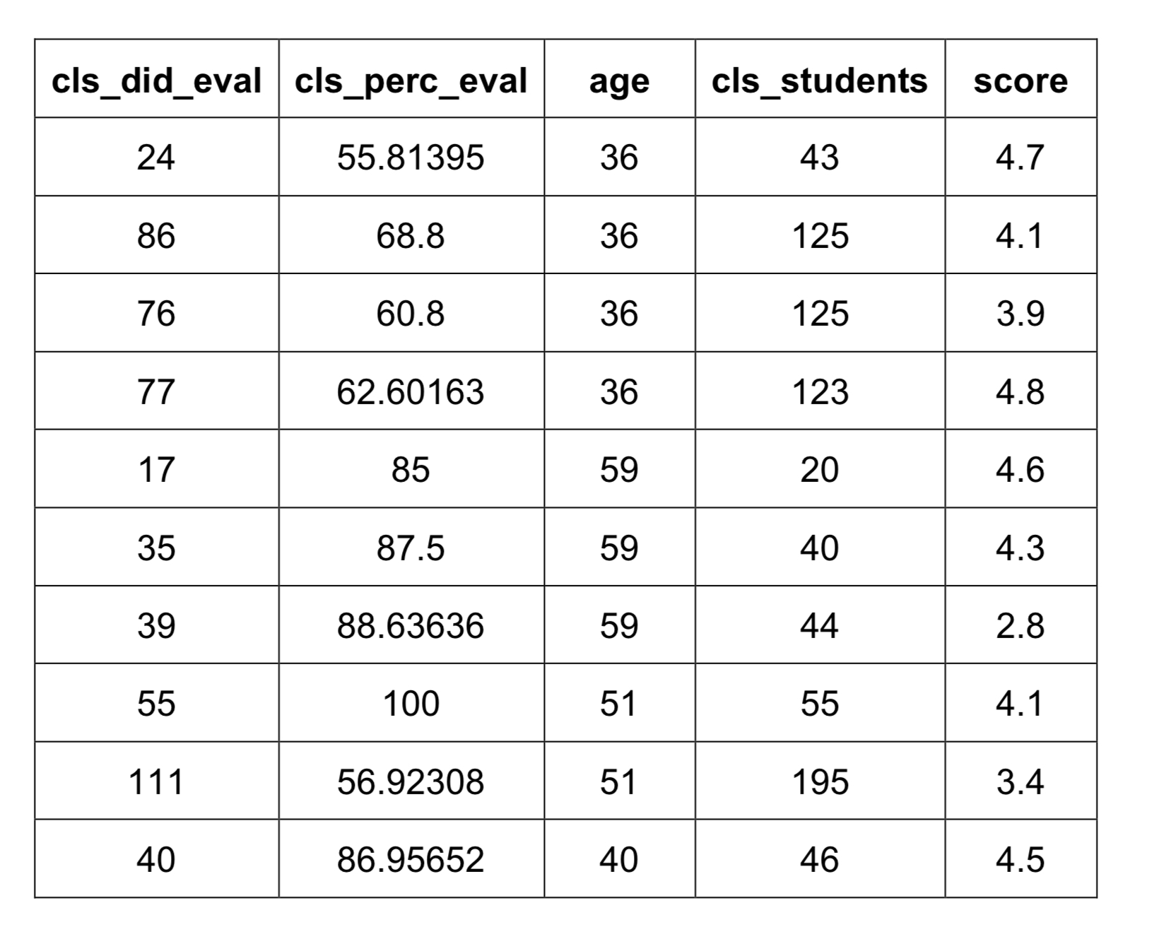
In this in-class activity, we will investigate the question: In general, what percentage of students completes course evaluations? To do so, we will use the evals dataset, which contains information collected from student evaluations for a sample of 463 courses taught by 94 professors at The University of Texas at Austin. Each row has a different course, and the columns have information about the professor and summaries from the evaluations. The first 10 observations of the selected variables within the “Teaching Evaluations” dataset are displayed in the following table.

The following variables are used in this analysis:

clsdideval: Number of students who completed evaluations

clsperceval: Percentage of students who completed evaluations

*age:*Age of professor in years \n cls_students: Total number of students in the course

score: Average professor evaluation score (1 to 5, where 1 is the lowest and 5 is the highest)

2) When looking at course evaluations, it’s important to understand how many students in the class completed the evaluation. There are two variables in the dataset that capture evaluation completion: clsdideval and clsperceval.

Which variable is more appropriate to help us understand whether the course evaluations generally represent the views of all the students in the course or just a few students? Explain.

The class number or class percentage because it gives us a number of people who participated and completed the evaluation.

3) Go to the Describing and Exploring Quantitative Variables tool at https://dcmathpathways.shinyapps.io/EDAquantitative/. Select the dataset “Teaching Evaluations – Percent Complete” to make a histogram of the distribution of clsperc_eval, the percentage of students who completed the course evaluations. Use bin width = 5. Sketch or capture a screenshot of your histogram below.

4) Use the histogram from Question 3 to answer the following questions.

Part A: In how many courses did all students complete the course evaluations?

In 10 courses, the students completed the course evaluations. (24 students)

Part B: About what proportion of courses had a completion rate between 60% (inclusive) and 80% (not inclusive)?

4/10 courses full in between the 60%-80% completion rate. Therefore, 40% oof the courses had a completion rate of between 60-80 percent. (165 students)

Part C: Based on these data, would it be more unusual for a course to have a completion rate less 70% or greater than 70%? Explain. Remember, if you are using the app, you can hover over the bar to get the exact counts.

It has a 50/50 chance of the course having a 70% completion rate.

So far, we’ve been able to use the histogram to answer questions about the distribution of clsperceval. The answers to these questions give us some information about the data; however, they do not give us a broad view of the overall distribution of the variable. In addition to visualizing the distribution with a graphical display, we can use common statistical language to describe the distribution. Before diving into the details, let's consider why we might want to use words to describe a distribution.

5) As a group, discuss why it is useful to include a written/verbal description of the features of a distribution in addition to the graphical display.

It helps us give more information and perspective on the study A graph would only show 2 variables, so an additional description will help make out what the study is observing.

6) Describe the shape of the distribution of clsperceval, the percentage of students who completed the course evaluations. If necessary, refer to the Describing Distributions section at the end of this activity for details about how to describe a distribution.

Skewed to the left.

7) What is the approximate center of the distribution of clsperceval, the percentage of students who completed the course evaluations?

74.7 is the mean of the graph.

8) The spread is a measure of how much the values in a dataset tend to differ from one another. One way we can describe the spread is by finding the minimum andmaximum values in the data and calculating the difference between them. This difference is called the ==range==****.

Part A: Use the range to describe the spread of clsperceval, the percentage of students who completed the course evaluations. Note that the web app provides values of the minimum and maximum.

The spread is the range of the graph which is 100.

Part B: Why might the range calculated in Part A be a potentially misleading measure of the spread of the distribution of clsperceval?

Due to outliers points.

9) Are there any outliers in the distribution of clsperceval, the percentage of students who completed the course evaluations? If so, briefly describe the outliers. If necessary, refer to the Describing Distributions section at the end of this activity for details about how to describe outliers.

3 points around 10 and 20

10) Now let’s use the features introduced in Questions 5–8 to describe the distribution of the following variables:

age**:** Age of professor in years \n Dataset = “Teaching Evaluations – Age”

cls_students: Total number of students in the course Dataset = “Teaching Evaluations – Students”

score: Average professor evaluation score (1 to 5, where 1 is the lowest) Dataset = “Teaching Evaluations – Scores”

Assign one variable to each group member.

Part A: For your assigned variable: (1) make a histogram of the distribution using the default bin width, and (2) describe the distribution, including the shape, center, spread, and presence of outliers.

Uniform

Part B: Have each group member share the description of their distribution with their group. As the other group members share, try to sketch the distributions based on their descriptions.