AP Precalculus Unit 1

1.1 - Change in Tandem

• Function - a mathematical relation that maps a set of input values to a set of output values.

  • Each input value must have exactly 1 OUTPUT VALUE

  • The set of input values of a function is called the domain, and is the independent variable.

  • The set of output values of a function is called the range, and is the dependent variable.

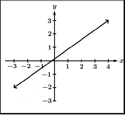
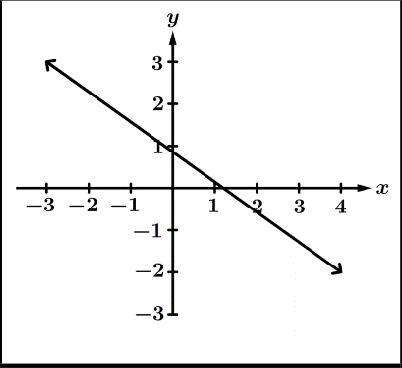
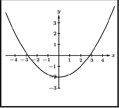
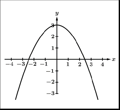
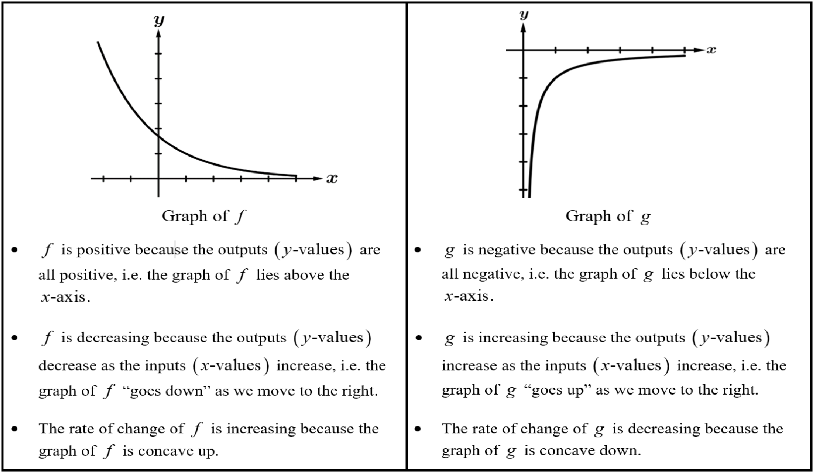
  • Function f is positive when the graph of f lies above the x-axis

  • Function f is negative when the graph of f lies below the x-axis

Graphical Behavior of Functions

Increasing	Decreasing	Concave Up	Concave Down
as the input values increase, the output values always increase.	as the input values increase, the output values always decrease	the rate of change* is increasing	the rate of change* is decreasing

*rate of change refers to the slope

1.2 - Rate of Change

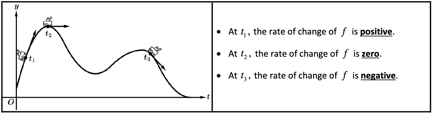
• Rate of Change at a Point

  • At the instant (point) when you are at the top of a peak or the valley, you are not moving up or down. At these points the rate of change is neither positive nor negative; the rate of change is zero

• Average Rate of Change (AROC)

  • The average rate of change of a function over an interval is the constant rate of change that yields the same change in the output values as the function yielded on that interval. It is the ratio of the change in output values to the change in the input values over that interval.

    \frac{f\left(b\right)-f\left(a\right)}{b-a}

On the interval from t = a with units to t = b with units, the function in context is increasing/decreasing on average at a rate of average rate of change with units.

1.3 - Rate of Change of Linear and Quadratic Functions

• Linear Functions

  • For any linear function, the average rate of change over any length input - value interval is constant.

• Concavity

  • Concave up - the average rate of change over the equal length input value intervals is increasing for all small length intervals.

  • Concave down - the average rate of change over the equal length input value intervals is decreasing for all small length intervals.

1.4 - Polynomial Functions and Rate of Change

• Polynomial Functions

  • A polynomial function is any function representation equivalent to the analytical form: p\left(x\right)=a_{n}x^{n}+a_{n-1}x^{n-1}+a_{n-2}x^{n-2}+\ldots+a_2x^2+a_1x+a_0

  • Leading Term: a_{n}x^{n} Degree: n Leading Coefficient: a_{n}

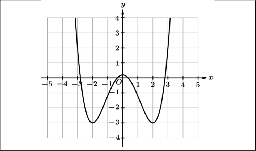
• Extrema

  • The extrema of a graph are the minimums and maximums of a function.

  • Polynomials of an even degree must have either a global maximum or a global minimum

Relative Extrema (Local)	Absolute Extrema (Global)
A polynomial has a relative minimum/maximum where it switches between decreasing and increasing (or at an endpoint if the polynomial has a restricted domain).	Of all local maxima, the greatest is called the absolute maximum. The least of all local minima is called the absolute minimum.

• Points of Inflection

  • a point of inflection occurs when a function changes from concave up to concave down or from concave down to concave up

  • At a point of inflection, the rate of change of a function changes from increasing to decreasing or from decreasing to increasing,

1.5 - Polynomial Functions and Complex Zeros

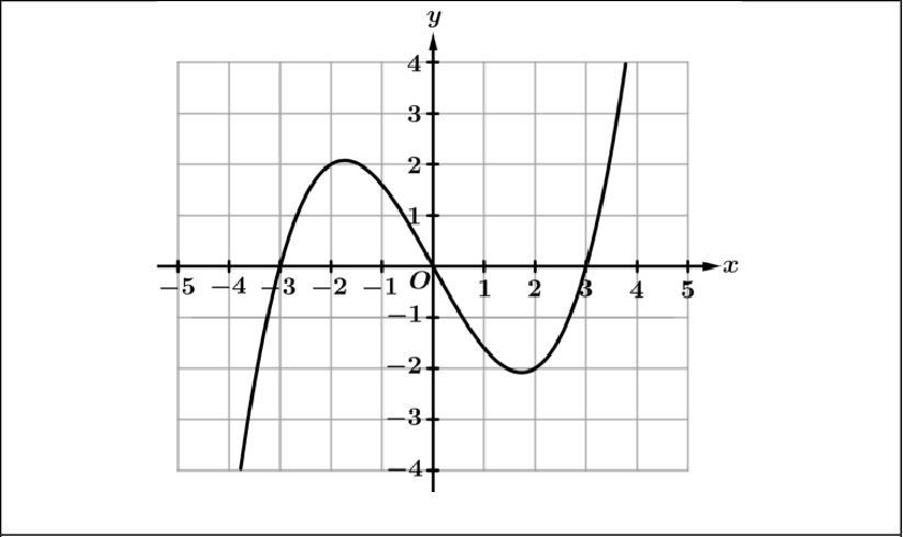
• Zeros of Polynomial Functions

  • Given a polynomial function p(x), if p(a) = 0, then a is zero or root of p(x).

  • If a is a real number, then if x = a is a zero of p, the (x - a) is a linear factor of p.

• Repeated Zeros (Multiplicity)

  • if a linear factor (x - a) is repeated n times, the corresponding zero of the polynomial has a multiplicity of n.

  • The multiplicity of a zero is the degree of its factor.

  • The graph of a polynomial will always be tangent to the x-axis at any zero with an even multiplicity.

  • The graph of a polynomial will always have a POI at the x-axis of any zero with an odd multiplicity.

• Complex Roots

  • some polynomials have roots that contain an imaginary number. This means they will not be seen on the graph.

  • All imaginary roots come in pairs. If a+bi is a root of f(x), then so is a-bi. These are called conjugate pairs.

• Fundamental Theorem of Algebra

  • a polynomial of degree n has exactly n complex zeros when counting multiplicities.

• Solving Nonlinear Inequalities (Polynomials)

  1. Solve f(x)=0.

  2. Creat a sign chart with the solutions from Step 1

  3. Test values in each interval to see if the values in the interval are positive or negative.

  4. Interpret the sign chart to answer the given inequality from the problem.

• Determining the Degree a Polynomial Given a Table of Values

  • if given a table of values with equal length input intervals, we can determine the degree of a polynomial by examining successive difference in the output values. The number of successive difference needed for the difference to be constant is equal to the degree of n of the polynomial.

Even Functions	Odd Functions
An even function is symmetric over the y - axis. f(-x) = f(x)	An odd function is symmetric about the origin. g(-x) = -g(x)
f\left(x\right)=x^4-8x^2+1	g\left(x\right)=x^3-9x

1.6 - Polynomial Functions and End Behavior

• End Behavior

  • The end behavior of a function is describes how a function changes as it moves infinitely to the right and left.

  • End behavior is what happens to the values of y as x increases or decreases without bound.

• End Behaviour and Limit Notation

• Polynomial End Behavior

  • when finding the end behavior of a polynomial equation, start with the right side

  • Right Side

    1. Goes up if the leading coefficient is positive

    2. Goes down if the leading coefficient is negative

  • Left Side

    1. Goes in the same direction as the right if the degree is even

    2. Goes in the opposite direction as the right if the degree is odd

1.7 - Rational Functions and End Behavior

• Rational Function

  • the quotient (fraction) of two polynomials

  • y=\frac{f\left(x\right)}{g\left(x\right)} where f(x) and g(x) are both polynomials, and g\left(x\right)\ne0

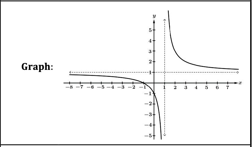
• End Behavior of a Rational Function

  • The end behavior of a rational function is determined by the leading terms of the numerator and denominator

f\left(x\right)=\frac{ax^{n}}{bx^{d}}

• Case 1 - The leading terms have the same degree (n = d)

  • Result - f(x) has a horizontal asymptote: y = \frac{a}{b}

• Case 2 - The denominator dominates the numerator \left(n<d\right)

  • Result - f(x) has a horizontal asymptote: y = 0

• Case 3 - The numerator dominates the denominator \left(n>d\right)

  • Result: f(x) has the end behavior of the polynomial y=\frac{a}{b}x^{n-d}

  • if the degree of the numerator is exactly 1 more than the degree of the denominator, then f(x) has a slant (oblique) asymptote.

  Case 1: N < D	Case 2: N = D	Case 3: N > D
  y = 0	y = \frac{a}{b}	No HA - Oblique (or other)

  • If the degree of the numerator if greater than the degree of the denominator, if nothing cancel, use long division to find the oblique asymptote (slant).

• Finding Oblique Asymptotes 

  1. Cancel any factors, if possible

  2. Perform Long Division

  3. The Quotient is the Oblique Asymptote: y=mx + b

• Slant Asymptotes

  • If the degree of the numerator is exactly 1 great than the degree of the denominator, a rational function will have a slant asymptote thats is parallel to the ratio of leading terms.

  • f\left(x\right)=\frac{ax^{n}+\ldots+c_1}{bx^{d}+\ldots+c_2} where ax^{n} and bx^{d} are the leading terms and n = d + 1,

  • f(x) has a slant asymptote parallel to the line y=\frac{a}{b}x

1.8 Rational Functions and Zeros

• 2 Important Traits of a Rational Function

  • let f\left(x\right)=\frac{g\left(x\right)}{h\left(x\right)} where g(x) an h(x) have no factor in common

  • f(x) has zeros when g(x) = 0

  • f(x) is undefined when h(x) = 0

• Solving Rational Inequalities

  1. Make sure the inequality has 0 on the other side

  2. Make sure f\left(x\right)=\frac{g\left(x\right)}{h\left(x\right)} (make sure you have a single rational function)

  3. Set g(x) = 0 and h(x) = 0 to find values to include on the sign chart (make sure to factor)

  4. Create a sign chart with all value from Step 3

  5. Be careful to mark the value where h(x) = 0 so that we NEVER include those values in our solution.

  6. Test values in each interval to see if the values in the interval are + or -

  7. Interpret the sign chart to answer the given inequality from the problem.

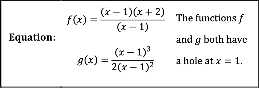
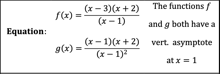
1.9/1.10 - Rational Functions and Vertical Asymptotes/Holes

• Rational functions have restrictions on their domain, because we cannot divide by 0, so consider any x values where g(x) = 0 and restrict them from the domain.

• These x values will be the location of either a vertical asymptote or a removable discontinuity (hole) in the graph.

• Vertical Asymptotes and Holes

  • A hole occurs when the factor in the denominator cancels out with the factors in the numerator.

  • A vertical asymptote occurs when a factor in the denominator cannot cancel out with factor in the numerator

Holes	Vertical Asymptote
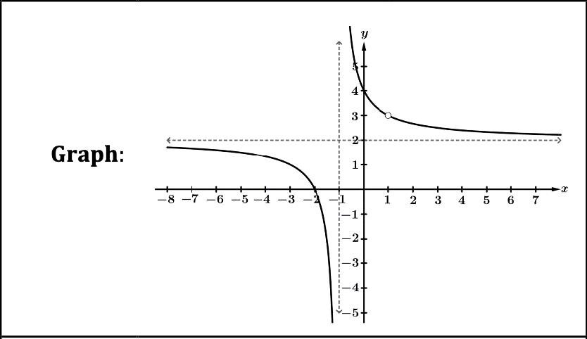The graph has a hole at x = 1	The graph above has a vertical asymptote at x = 1
\lim_{x\to1^{-}}f\left(x\right)=3 \lim_{x\to1^{+}}f\left(x\right)=3	\lim_{x\to1^{-}}f\left(x\right)=-\infty \lim_{x\to1^{+}}f\left(x\right)=\infty

1.11 - Equivalent Representations of Polynomial and Rational Expressions

• To find the equation of a slant asymptote we will us long division

• Long Division

  • If f(x) and g(x) are polynomials, the \frac{f\left(x\right)}{g\left(x\right)}=g\left(x\right)q\left(x\right)+r\left(x\right) , where q is the quotient, r is the remainder, and the degree of r is less than the degree of g.

• Pascal’s Triangle and the Binomial Theorem

  The Binomial Theorem

  \left(a+b\right)^{n}=\left(\frac{n}{0}\right)a^{n}+\left(\frac{n}{1}\right)a^{n-1}b^1+\left(\frac{n}{2}\right)a^{n-2}b^2+\ldots+\left(\frac{n}{n-1}\right)a^1b^{n-1}+\left(\frac{n}{n}\right)b^{n}

  1. When expanding a binomial expression, the “a” begins with degree n and the “b” term begins with a degree of 0.

  2. As you expand the binomial expression, the degree of “a” decrease by one each term while the degree of “b” increases by on each term (until the term “b” has degree n).

  3. Use Pascal’s Triangle to find the values of the coefficients \left(\frac{n}{0}\right),\left(\frac{n}{1}\right),\left(\frac{n}{2}\right),\ldots in our expansion

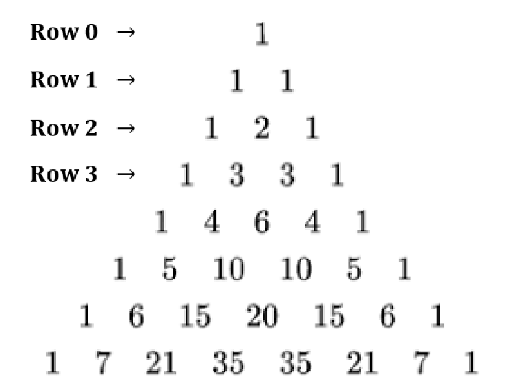
• The value of \left(\frac{n}{r}\right) corresponds with the rth element of the nth row in Pascal’s triangle.

The first number in each row is the 0th element of that row. nn n

1.12 - Transformations of Functions

• H(horizontal)I(inside)V(vertical)O(outside)

  • any transformations that affect the x values will do the opposite of what it looks like to the x values

  • any transformations that affect the y values will do exactly what it looks like to the y values

1.13 - Function Model Selection and Assumption Articulation

• Determining a function based on a data table

  • If over equal-length input values (ex. 1,2,3 or 2,4,6), the output values have a common first difference, the table is a linear function

  • If over equal-length input values, the output values have a common second difference, the table is a quadratic function

  • If over equal-length input values , the output values have a common third difference, the table is a cubic function

• Determining a function based on geometry

  • Perimeter - linear function

  • Area - quadratic function

  • Volume - cubic function

• Restricted Domain and Range

  • domain will be the furthest x value that fits the context of the model

  • range will be the maximum and minimum y value that fits the context of the model

• Piecewise Functions

  • a function whose domain is partitioned into several intervals

• Inversely Proportional

  • when one variable increases the other decreases, and vice versa

1.14 - Function Model Construction and Application

• Building Regressions Models on the Graphing Calculator

  1. Press “stat” and select “edit”

  2. enter the data into lists with L1 = x and L2 = y

  3. In the “stat” arrow to the “CALC” menu

  4. Enter the desired regression model

     • to Store RegEQ; enter Y1 (press “alpha” and then “trace”)

• Selecting an Appropriate Model Type

  • Linear Model: roughly constant rates of change

  • Quadratic Model: roughly linear rates of change or roughly symmetric with a single maximum/minimum or context involving area

• Residuals

  • Residual = Actual Value - Predicted Value