AP Precalculus Guide (new version)
Unit 1
1.1 - Change in Tandem
A function is a mathematical relation that maps a set of input values to a set of output values such that each input value is mapped to exactly 1 output value
Positive Function - the output values are above 0
Negative Function - the output values are below 0
Increasing function if…
Verbally: as the input values increase, the output values always increase
Analytically: for all a and b in the interval ___, if a < b, then f(a) < f(b)
Decreasing function if…
Verbally: as the input values increase, the output value always decreases
Analytically: for all a and b in the interval ___, if a < b then f(a) > f(b)
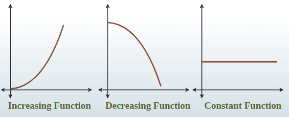
Zero: when the output value is zero
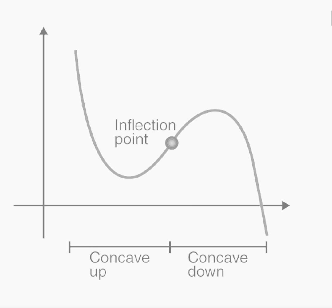
Concave up: bowl facing UP → slope increasing
Concave down: bowl facing DOWN → slope decreasing
Point of Inflection: point where the concavity changes
Justification on stating whether or not the function is increasing or decreasing…
x | 4 | 6 | 7 | 10 |
f(x) | 1 | 1.01 | 1.04 | 1.06 |
The function f is increasing on the interval 4 < x < 10 or (4, 10) because for all a and b values, if a < b, then f(a) < f(b)
1.2 - Rates of Change
rate of change = slope
Rate of Change of a point
Ex. Estimate the rate of change at x = 1 for the function f(x) = -½x² + 3x - ½
Get as close as you can to the point (at least 3 decimal places)
(1, 2) & (1.001, 2.0019995)
Now calculate the slope
(2.0019995 - 2) ÷ (1.001 - 1) = 1.9995 ≈ 2
Positive ROC - indicates that as one quantity increases or decreases the other quantity does the same (same as if it were to say a function is increasing)
Negative ROC - indicates that as one quantity increases, the other decreases (same as if it were to say a function is decreasing)
1.3 - Rates of Change in Linear and Quadratic Functions
Average Rate of Change = Slope of a SECANT Line (calculates overall change in a quantity across a given interval)
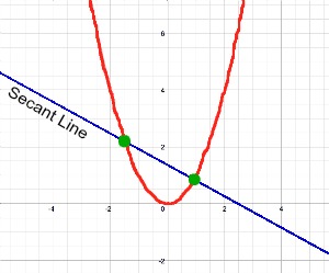
average rate of change = f(a) - f(b) / a - b
The average rate of change for a linear function is constant. Regardless of the input-value interval length, the average rate of change always stays the same
Does not matter where you pick your points, the slope is always the same
x | 15 | 16 | 17 | 18 | 19 |
f(x) | 18 | 20 | 22 | 24 | 26 |
NOTE: linear functions only have an increase/decrease in the y values, meanwhile quadratics have an increase/decrease in the average rate of change (the amount of differences is the degree)
The amount of differences you get from this indicates the degree. 1 is linear, 2 is quadratic, 3 is cubic, 4 is quartic, 5 is quintic, etc.
The average rate of change for a quadratic doesn’t stay the same. For consecutive equal-length input-value intervals, the average rate of change of the rate of change of a quadratic function is constant.
here the x is going up by one (15 +1 = 16; 16 +1 = 17)
x | 15 | 16 | 17 | 18 | 19 |
f(x) | 18 | 20 | 20 | 18 | 14 |
The rate of change of the rate of change: what is the change in the slope/ROC (This will always be 0 for linear functions)
here the bottom is varying (18 + 2 = 20; 20 + 0 = 20; 20 - 2 = 18; 18 - 4 = 14)
Then you would do that again to find a commonality (+2, 0, -2, -4) → ( 0 - 2 = -2; -2 - 0 = -2; -4 - (-2) = -2)
Which means the rate of change of the rate of change is -2
The function is concave down because the rate of change is decreasing over equal length input intervals
Example problem on quiz:
The function p is given by p(x) = g(x + 1) - g(x). If p(x) = 2, which of the following statements must be true?
g(x + 1) - g(x) is really the slope (y2 [which is f(x + 1)] - y1 [which is f(x)]) / 1
p(x) = 2 means that the slope is 2
This means the graph always has a positive slope and that because p is positive and constant, g is increasing
Confusing Terms
Positive Rate of Change | Negative Rate of Change |
The independent variable increases, the dependent variable also increases | As the independent variable increases the dependent variable decreases |
Increasing Rate of Change | Decreasing Rate of Change |
The rate of change (slope) itself is increasing Ex. (car speed goes from 20 to 30 in one hour and 30 to 70 in the next hour) | The rate of change (slope) itself is decreasing Ex. (car speed increases from 30 to 40 in 1 hour and then to 45 in the next hour, the acceleration is decreasing) |
Positive Average Rate of Change | Negative Average Rate of Change |
Whether the rate of change between an interval or 2 points (secant line) is positive | Whether the rate of change between an interval or 2 points (secant line) is negative |
Increasing Average Rate of Change | Decreasing Average Rate of Change |
The rate of change over an interval itself is increasing Ex. (In a 3 hour period, a car goes 10 mph at 1 hour, 15 mph a 2 hours and 20 mph at 3 hours, the aroc of the speed is increasing) | The rate of change over an interval itself is decreasing Ex. (In a 3 hour period, a car goes 20 mph at 1 hour, 15 mph a 2 hours and 10 mph at 3 hours, the aroc of the speed is decreasing) |
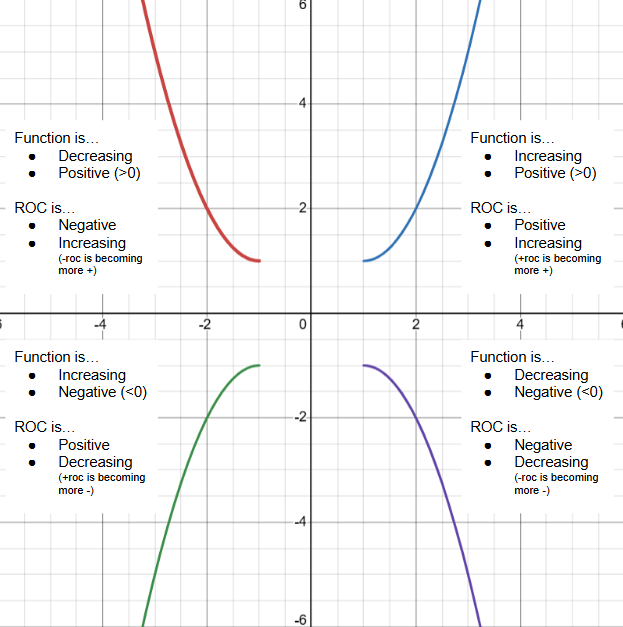
Increasing + Positive ROC | Increasing + Negative ROC |
→ The function is increasing → The graph is concave up | → The function is decreasing → The graph is concave up |
Decreasing + Positive ROC | Decreasing + Negative ROC |
→ The function is increasing → The graph is concave down | → The function is decreasing → The graph is concave down |
Increasing / Decreasing ROC → The graph is concave Up / Down
Positive / Negative ROC → The function is Increasing / Decreasing (± slope; imagine a positive or negative linear line)
1.4 - Polynomial Functions and Rates of Change
Polynomial
p(x) = anxn + an-1xn-1 + an-2xn-2 + … + a1x2 + a1x + a0
anxn is the leading term | n is the degree | an is the leading coefficient
Local / Relative Maximum - if the polynomial switches from increasing to decreasing
Local / Relative Minimum - if the polynomial switches from decreasing to increasing
an included endpoint of a polynomial with a restricted domain may also be the local minimum or maximum
Global Maximum - the greatest of the local maximums (If it goes to infinity, there is none)
Global Minimum - the least of the local minimums
Two Zeros = if you have 2 zeros of a polynomial, there must be at least 1 local extrema between the two
Even degree = absolute extreme
Positive leading coefficient = absolute minimum
Negative leading coefficient = absolute maximum
1.5A - Polynomial Functions and Complex Zeros & 1.5B - Even and Odd Polynomials
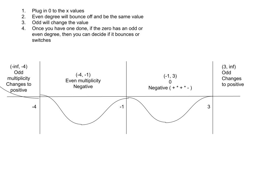
If the real zero, a, of (x - a), has an even multiplicity, then the graph will bounce off the x-axis
Example:
Given the function: (x + 1)2(x - 3)3(x + 4)1
Complex Zeros - non-real zeros that will always come in pairs (Ex. 3 ± 2i)
a ± bi
Even functions = symmetrical over the y-axis
has the property f(-x) = f(x)
You can prove that the function is even by substituting in -x and see if you get the same original function
Ex. f(x) = x6 - 4x2 → f(-x) = (-x)6 - 4(-x)2 → f(-x) = x6 - 4x2
Odd functions = symmetrical over the origin
has the property f(-x) = -f(x)
1.6 - Polynomial Functions and End Behavior
The left or right side of a polynomial will either go up or down.
The limit expresses the end behavior of a function.
The Left Side
The x values are approaching negative ∞
lim x → -∞ f(x)
The Right Side
The x values are approaching positive ∞
lim x → ∞ f(x)
Left Side | Right Side | |
Up | ||
Down |
Left side x → -∞ | Right Side x → ∞ | |
Even degree and Positive leading coefficient | ||
Even degree and Negative leading coefficient |
Even degree means that the left and right side will behave the same
Odd degree means that the left and right side will behave opposite
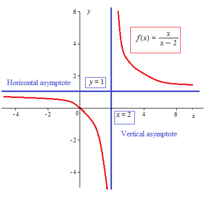
1.7 - Rational Functions & End Behavior
Rational Function - the ratio of two polynomials where the polynomial in the denominator cannot equal 0
Usually can be described as:
Labeling some of the properties of the function:
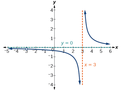
Domain: (-∞, -3) U (-3, 3) U (3, ∞) There is a hole and vertical asymptote
limx → -∞ f(x) = 0 | limx → ∞ f(x) = 0
0 is the horizontal asymptote because both limits approach this number
For inputs with a larger magnitude, the polynomial in the denominator dominates the polynomial in the numerator
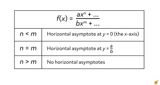
Ways to remember:
BOBO BOTNA EATS DC
BOBO - Bigger on bottom = 0 (BOB0)
BOTNA - Bigger on top = No Asymptote (BotNA)
EATS DC - Exponents Are The Same = Divide Coefficients (EATSDC)
1.8 - Rational Functions & Zeros
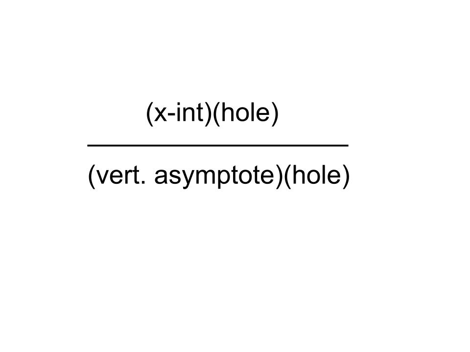
When there is an unfactored polynomial in a rational function, try to factor both numerator and denominator to make it easier to see holes and asymptotes
This is a helpful equation when working with a polynomial that is both factored on the numerator and denominator: (x-int)(hole) / (hole)(vertical asymptote)
Example function:
X intercepts (zeros) will be any factors on the numerator that aren’t holes
(x + 3); so that means that there is an x-intercept at x = -3
Holes will appear on both the numerator and denominator (This is the value you cannot plug into the equation)
(x - 2) / (x - 2); meaning that x = 2 does not exist
Vertical asymptotes are any factors that aren’t holes left in the denominator
(x + 4); so that means that there is a vertical asymptote at x = -4
1.9 - Rational Functions & Vertical Asymptotes
Finding the limit as x approaches a number/asymptote
2- means approaching the vertical asymptote on the left side from left to right
2+ means approaching the vertical asymptote on the right side from right to left
Order of dominance (VA > Hole > 0)
Hole > 0
If there is a zero with a hole, then there will be no zero, but a hole instead where the zero would be
Ex. means that there will be a hole at x = -1 instead of a zero because there is a hole of (x + 1)
Vertical Asymptote > Hole
If there is a vertical asymptote the same as a hole, then that hole will be a vertical asymptote
Ex. means that there is a vertical asymptote at x = -1 instead of a hole because there is a vertical asymptote of (x + 1)
1.10 - Rational Functions & Holes
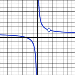
Writing limits for holes:
From the left:
As x approaches 3 from the left, f(x) approaches 2
From the right:
As x approaches 3 from the right, f(x) approaches 2
Using a Table to Determine Limits
x | 2.9 | 2.99 | 3 | 3.01 | 3.1 |
f(x) | 2.0345 | 2.0033 | undefined | 1.9967 | 1.9677 |
As you can see, the closer we get to 3, the closer the values get to 2
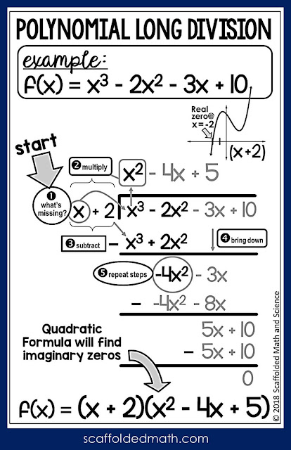
1.11A - Equivalent Representations & Binomial Theorem & 1.11B - Polynomial Long Division & Slant Asymptotes
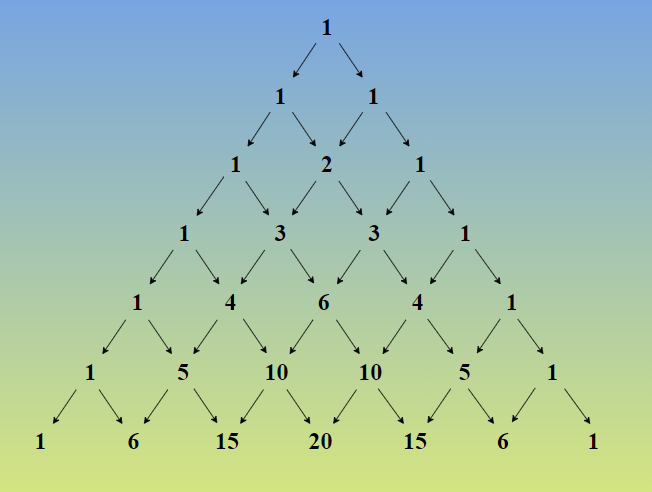
Using pascal’s triangle, you can expand binomials. The rows of pascal’s triangle start from 0 (the top) and so on.
For example, if you had (x + 3)4 then the row you would use would be → 1 4 6 4 1
Binomial Theorem:
The formula is (x + y)n where n would be the row #
(a+b)n = C1anb0 + C2an - 1b1 + C3an - 2b2 + … + Cn - 1a1bn - 1 + Cna0bn
C is the coefficient corresponding to the row in pascal’s triangle
n is the power
Using the numbers in pascal’s triangle, expand the polynomial
As the power of x decreases, the power of y increases
Ex. (x + 5)3
1x350 + 3x251 + 3x152 + 1x053 → x³ + 15x² + 75x + 125
Slant Asymptote - When the degree of the numerator is one higher than the degree of the denominator
End behavior of slant asymptote:
Finding the asymptote of the slant asymptote with long division or synthetic division will give you the linear equation. The end behavior of that function (in this case, y = x + 1) is the end behavior of the rational function
Long Division
Long division can be used to divide any polynomial by another one
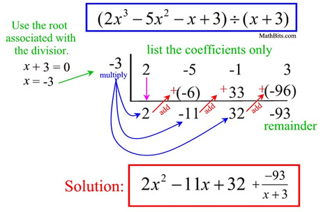
Synthetic Division:
Synthetic division can only be used when dividing a polynomial by a factor like (ax + b)
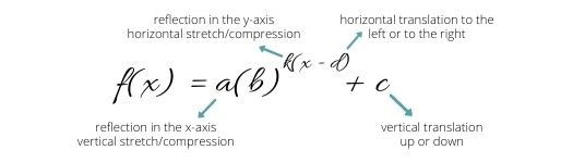
1.12 - Transformations of Functions
Vertical Translations (anything done outside of the function)
f(x) + d → up by d units
f(x) - d → down by d units
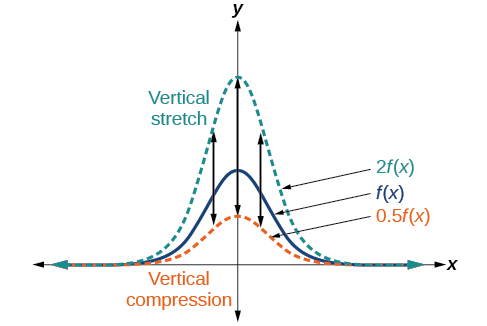
Vertical Dilations (anything done outside of the function)
a × f(x)
When doing a vertical dilation, only the y-values change, the x-values do not
Multiply the y-values by a
a > 1: vertical stretch
a < 1: vertical shrink
Horizontal Translations (anything done inside the function)
f(x - d) → right by d units
f(x + d) → left by d units
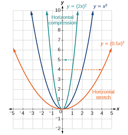
Horizontal Dilations (anything done inside the function)
f(bx)
b is inverted (if it was f(3x) that would be a horizontal dilation of 1/3)
When doing a horizontal dilation, only the x-values change, the y-values do not
Multiply the x-values by the inverse of b
1/b > 1: horizontal shrink
1/b < 1: horizontal stretch
Reflections
-f(x) → reflect over x-axis → vertical change
f(-x) → reflect over y-axis → horizontal change
Transformations Numerically
x | 0 | 1 | 2 | 3 | 4 |
f(x) | -20 | -12 | 0 | 8 | 14 |
Ex. let g(x) = 3f(x - 2) + 1, find g(3)
g(x) = 3f(x - 2) + 1 → set up equation
g(3) = 3f(3 - 2) + 1 → plug in the 3 for x in the modified equation
g(3) = 3f(1) + 1 → simplify
g(3) = 3(-12) + 1 → find what f(1) is and substitute that in
g(3) = -35 → solve
Transformations through domain & range
Ex. Given the graph for f has a domain of [-4, 3] and a range of (3, 9]. Let g(x) = -f(x + 5) + 2.
f(x)
Domain: [-4, 3]
Range: (3, 9]
g(x)
Domain: [-4 - 5, 3 - 5] → [-9, -2]
f(x + 5) → move left 5 → subtract 5 from the domain
Range: (3 * -1, 9 * -1] → (-3 + 2, -9 + 2] → (-1, -7]
Do the inversions and dilations first then the translations
Transformations Algebraically
Ex. Given f(x) = x² - 3x + 2, let g(x) = f(x - 3) + 2, find g(x)
g(x) = f(x - 3) + 2 → set up equation
[(x - 3)² - 3(x - 3) + 2] + 2 → substitute the input values in g(x) for x in f(x)
(x² - 6x + 9 - 3x + 9 + 2) + 2 → distribute
(x² - 9x + 20) + 2 → combining like terms
g(x) = x² - 9x + 22 → solved
1.13 - Function Model Selection
Perimeter will be linear
Area will be quadratic
Volume will be cubic
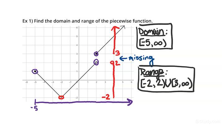
Restricted Domain & Range
Restricted domain and range is give between brackets and is usually given in a word problem or between a piece of a function
Piecewise Functions
Range of a piecewise function

1.14 Function Model Construction
Types of Regression
Linear
Quadratic
Cubic
Quartic
Exponential
Logarithmic
Logistic
Sine
Inversely Proportional
When something is inversely proportional, the equation y = k / x is used
k is some constant
Ex. The number of workers at a job is inversely proportional to the time it takes to complete a task. If there are 15 workers and it takes 20 minutes to do a task, then how many workers would it take to complete a task in 3 minutes?
n = k / t → number of workers = k / time
15 = k / 20 → set up equation to solve for k
k = 15 × 20 = 300 → solve for k
n = 300 / 3 → input k into new equation to solve for workers
n = 100 workers → it would take 100 workers to complete a task in 3 minutes
Piecewise Functions Algebraically
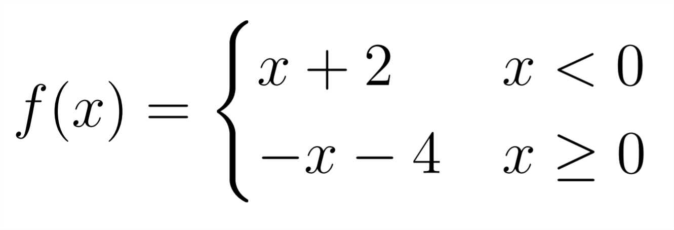
Piecewise functions can be shown like the image above. The function on the left is in the bounds of the inequality on the right.
Unit 2
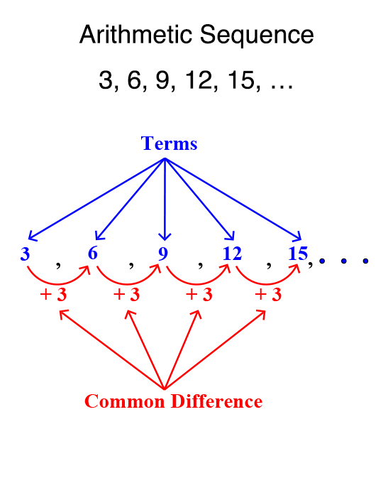
2.1 - Change in Arithmetic and Geometric Sequences
Sequence → an ordered list of numbers; each listed number is a term
Ex. {1, 3, 5, 7, 9, …} (… means it keeps going continuously)
1 would be the first term not the zero term
Arithmetic Sequences
Linear
If each successive term in a sequence has a common difference (constant ROC), the sequence is arithmetic
Equation for the nth term →
a0 is the initial value (zero term) and d is the common difference
Equation for any term →
ak is the kth term of the sequence
Geometric Sequence
Exponential
If each successive term in a sequence has a common ratio (constant proportional change) the sequence is geometric
If dividing is involved (for example, {4, 2, 1, …} is ÷2 each time), then the ratio will be multiplied by a fraction (÷2 → ×1/2)
Equation for the nth term →
g0 is the initial value (zero term) and r is the common ratio
Equation for any term →
gk is the kth term of the sequence
2.2 - Change in Linear and Exponential Functions
Linear Functions vs Arithmetic Sequences
They are basically the same, except when using a sequence vs a function, the domain and points are discrete, meaning the domain only includes specific points and not all numbers in between
The point (x1, y1) of a linear function is similar to (k, ak) of an arithmetic sequence
Slope-intercept form f(x) = b + mx | Arithmetic Sequence an = a0 + dn |
Point-slope form f(x) = y1 + m(x - x1) | A.S. for the kth term an = ak + d(n - k) |
Exponential Functions vs Geometric Sequences
Again, they are basically the same except with discrete points for the sequence
The point (x1, y1) of an exponential function is similar to (k, gk) of a geometric sequence
Exponential Function f(x) = abx | Geometric Sequence gn = g0rn |
Shifted Exponential Function f(x) = y1r(x - x1) | G.S. for the kth term gn = gkr(n - k) |
How each output value changes analytically
Arithmetic → Over equal-length input value intervals, if the output values of a function change at a constant rate, then the function is linear (adding the slope)
Geometric → Over equal-length input value intervals, if the output values of a function change proportionally, then the function is exponential (multiplying the ratio)
“Over equal-length input intervals” means that the x-values of the function or a table are increasing by a constant amount (ex. 1, 2, 3, 4 or 2, 4, 6, 8)
Finding whether a set of points is linear or exponential
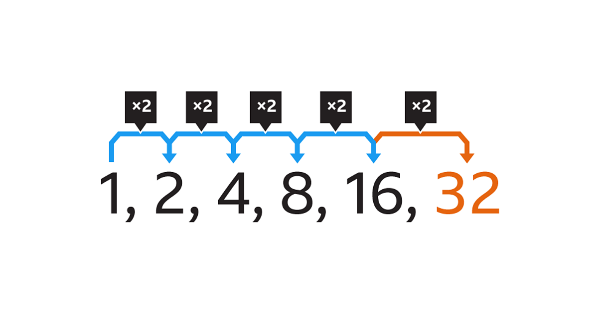
x | 5 | 6 | 7 |
f(x) | 8 | 16 | 32 |
Make sure the function is increasing over equal-length input intervals
Test to see whether the function is linear or exponential
Linear functions change by adding or subtracting a constant amount
Exponential functions change by multiplying or dividing a constant amount
This example is increasing x2 from 8-16 and 16-32
So this function is exponential because over equal-length intervals of 1, f(x) proportionally changes by a ratio of 2
If this was linear you could say, the function is linear because over equal-length input intervals of ___, f(x) has a constant rate of change of ___
Finding a common difference/ratio from a set of points
Common Difference
Given the points (a, b) & (c, d), you can find the common difference using the slope formula →
Common Ratio
1 | 2 | 3 |
4 | ? | 16 |
Find how many times r would have to be multiplied to get from 4 to 16 (in this case it is 2)
This means we would have to multiply 4 ⋅ r ⋅ r to get 16 → 4r² = 16
Then, you solve for r → r² = 16/4 = 4 → r = √4 = 2
So r = 2
OR… given the points (a, b) & (c, d), you can find the common ratio using this equation →
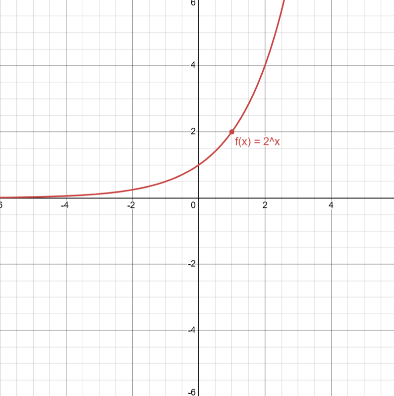
2.3 - Exponential Functions
General form of an exponential function → f(x) = abx
a = initial value
a ≠ 0 & b > 0
Exponential growth → when a > 0 & b > 1
Exponential decay → when a > 0 & 0 < b < 1
Determining exponential function based on output values
Ex. 3 × 3 × 3 × 3 × 6
a, the input value, will be the odd one out: 6
the rest are the common ratio multiplied by however many times
f(x) = 6(3)x where x = 4
Exponential Functions depending on parameters
a > 0; b > 1
 | a > 0; 0 < b < 1
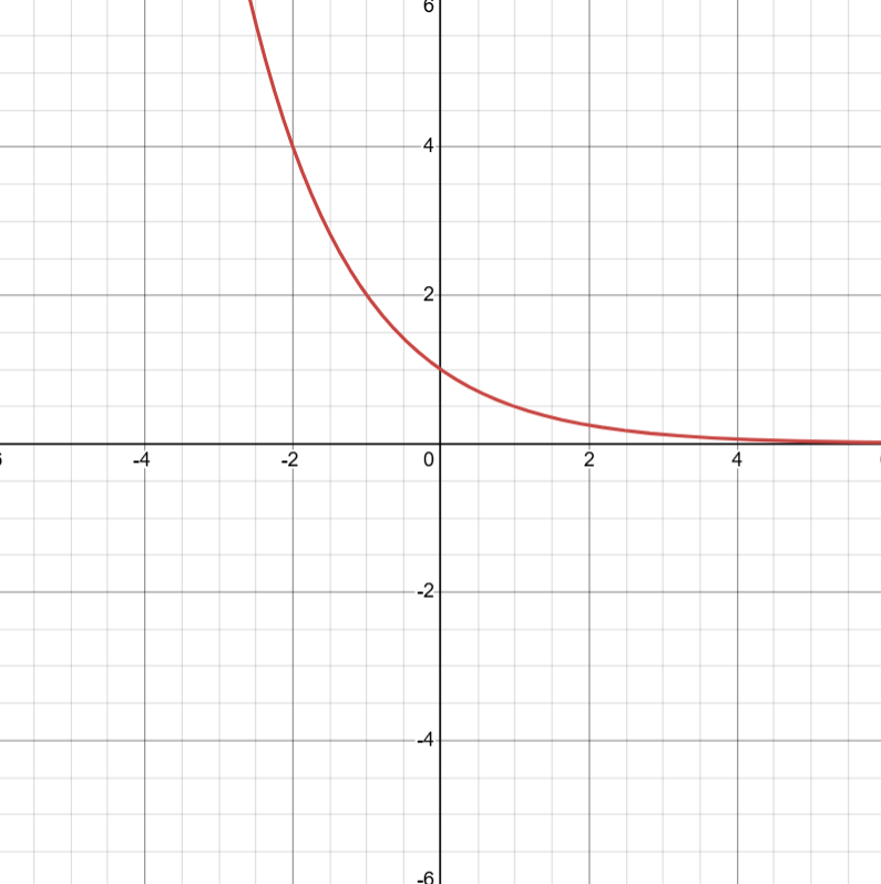 |
a < 0; b > 1
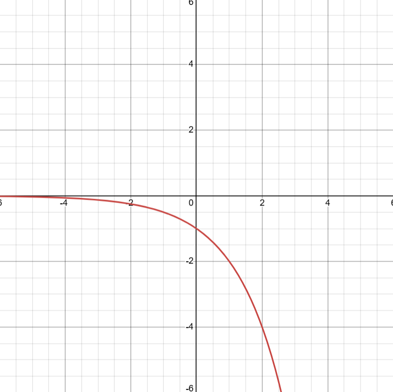 | a < 0; 0 < b < 1
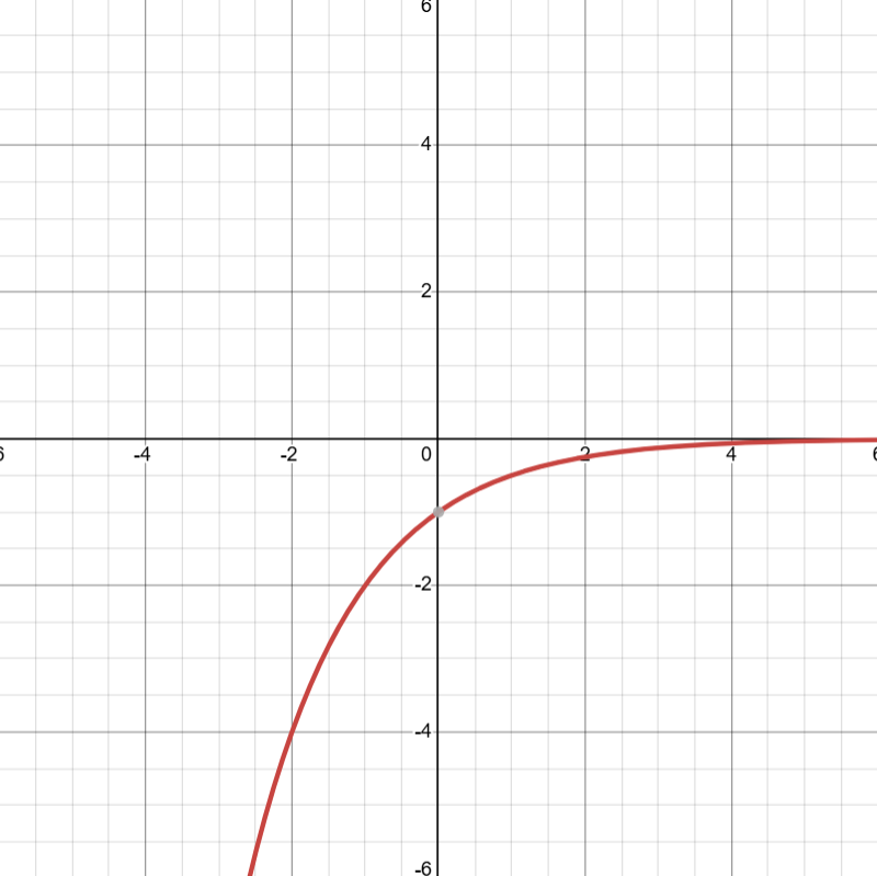 |
Characteristics of Exponential Functions
They are always increasing or decreasing
There is no extreme (except on closed intervals)
Their graphs are always concave up or concave down
They have no inflection points
If the input values increase or decrease without bound, the end-behavior can be expressed as
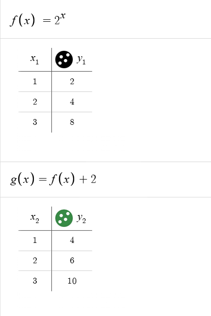
Additive Transformation of an Exponential Function
g(x) = f(x) + k
If the output values of g are proportional over equal-length input-value intervals, then f is exponential
Meaning that if g(x) has proportional output values, then f(x) will always be exponential
But if f(x) is proportional, that doesn’t mean g(x) will be proportional
2.4 - Exponential Function Manipulation
Negative Exponent Property →
Product Property →
Product Property →
Transformations of Exponential functions
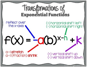
Horizontal Translations & Vertical Dilations
ac(b)x = bkbx = b(x + k)
Through the product property, when doing a horizontal translation, it is the same as doing a vertical dilation
Every horizontal translation of an exponential function, f(x) = b(x + k), is equivalent to a vertical dilation
Ex. 1(2)(x + 3) → 1 × 23(2x) → 8(2)x
Horizontal translation left by 3 units / Vertical dilation of 8 units
Horizontal Dilations
Every horizontal dilation of an exponential function, f(x) = b(cx), is equivalent to a change of base
(bc)x → bc and c ≠ 0
Ex. 23x → (23)x → 8x
The kth Root of b
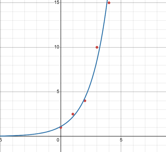
2.5 - Exponential Function Context & Data Modeling
Finding the exponential function in the form f(x) = abx + k through a table
x | 0 | 1 | 2 | 3 | 4 |
f(x) | 6 | 9 | 15 | 27 | 51 |
Find the ratio (b) (in this case b=2)
Find the differences
9-6 = +3; 15-9= +6; 27-15= +12; 51-27= +24
Then, you can find the ratio
3 × 2 = 6 × 2 = 12 × 2 = 24
Then find a and k by setting up a system of equations
6 = a(2)0 + k → 6 = a + k
9 = a(2)1 + k → 9 = 2a + k
9 = 2a + k
-6 = -a - k
a = 3
6 = 3 + k → k = 3
The number e
e ≈ 2.718…
The natural base e is often used as the base in exponential functions that model contextual scenarios
Percent Increase:
Start with the initial amount a and grow with a % increase
y = a(1 + %increase)x
Percent Decrease:
Start with the initial amount a and decay with a % decrease
y = a(1 - %decrease)x
Half-Life:
An initial amount a that shrinks by half every h
f(t) = a(1/2)t/h
Doubling time:
An initial amount a that doubles every d
f(t) = a(2)t/d
Equivalent Forms
If t represents the number of weeks, then the base of f(t) = (1.01)t indicates that the quantity increases by a factor of 1.01 every week
If you want the equation for every year, then that equation would look like this → (1.0152)t/52
This is because every 52 weeks, t = 52/52, means that it would account for 1 year
since we’re counting years, 1.0152 means that in 1 year, we’d have (1.01 × 1.01 × 1.01 … 1.01) → 52 times per year
So when t = 52 weeks / 52 (one year), 1.01 would’ve increased 52 times
If you wanted an equation for every day, then it would look like this → (1.011/7)t
This is because once t is > 7, the function will equal 1.01 which is the same as if it where (1.01)1 weeks
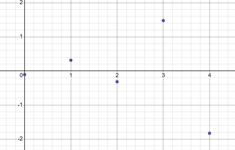
2.6 - Competing Function Model Validation
The only way to know what model fits an equation best is to use context clues
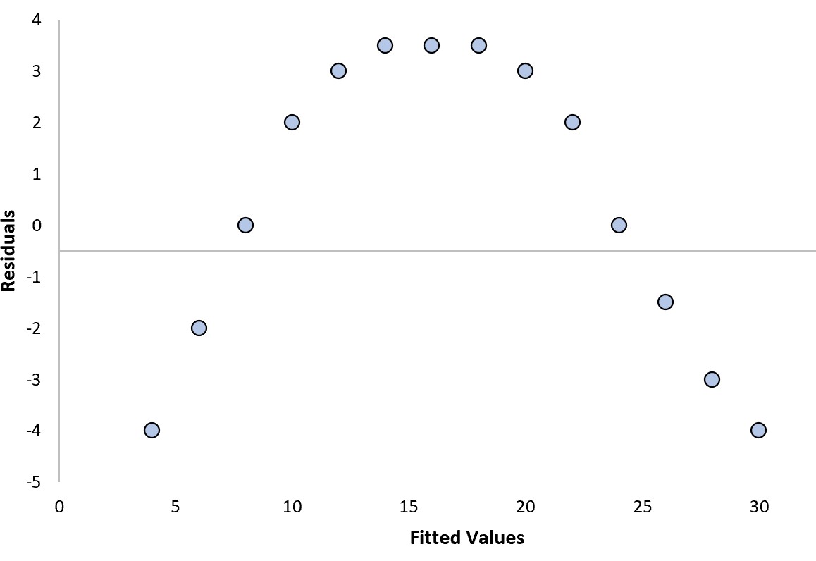
Residual Value - a measure of how much a regression curve vertically misses a data point
Residuals → Actual - Predicted (AP *remember RAP*)
The difference between the predicted and actual values is the error
Error → Predicted - Actual (PA *remember EPA*)
A positive error means that the model overestimated (you can see the y=0 line is above the point)
A negative error means that the model underestimated (you can see the y=0 line is below the point
Residual Plot Patterns
If there is a clear pattern in the residual plot, it is a bad regression model
2.7 - Composition of Functions
The composition of functions means we take one function and substitute it into the other function
f(g(x) or f ∘ g(x)
Ex. f(x) = 2x + 3; g(x) = 5x²; find f(g(5))
5(5)² → 5(25) → 125
2(125) + 3 = 253
Identity Function
When f(x) = x
then f(g(x)) = g(x)
Finding a Composed Function
f(x) = x² - 1 & g(x) = √x ; find f(g(x))
h(x) = (√x)² -1
h(x) = x - 1
Domain of a Composed Function
When finding the domain of a function h(x) = f(g(x)), there are 2 things to consider
because g(x) is the input, we can only use x-values in the domain of g
any restrictions on the domain of f(g(x)) must be included
Ex. problem above in Finding a Composed Function
g(x) is the input, so it can only be from [0, ∞)
and there are no restrictions in x - 1, so the domain is [0, ∞)
Decomposition of Functions
if there is a radical, one function can simply be √x (this applies with 1/x as well)
Ex. h(x) = √x³ + 1 ; find f(g(x))
f(x) = √x
g(x) = x³ + 1
Ex2. h(x) = 1/(x² + 1) ; find g(f(x))
f(x) = x² + 1
g(x) = 1/x
2.8 - Inverse Functions
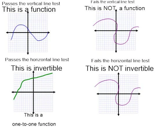
The inverse of a function is a reverse mapping of a function where (x, y) → (y, x)
They should reflect across the line y=x
If the graph turns (has a max/min) then it is no longer invertible because there will be output values that are the same for different input values
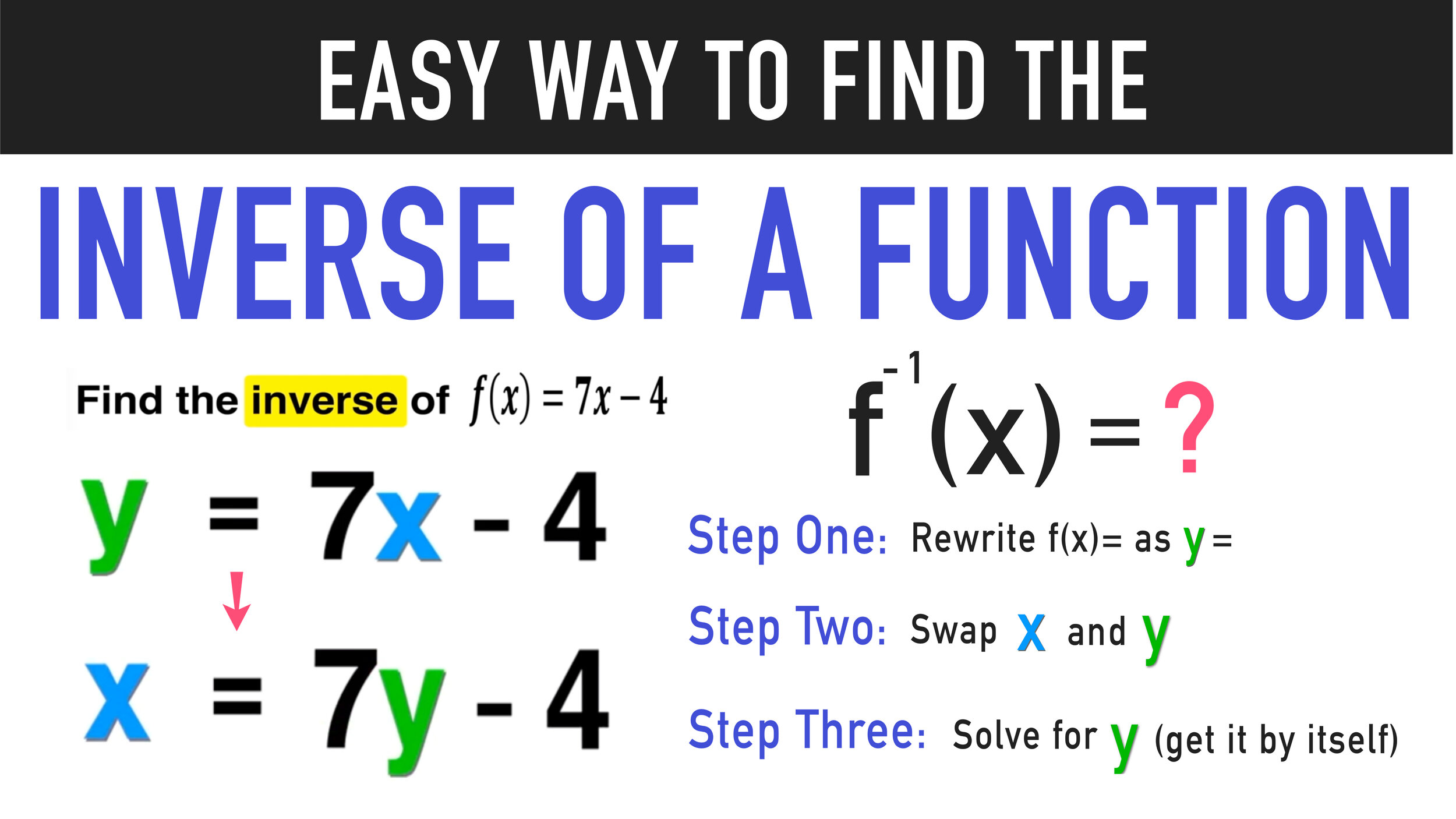
Find the Inverse of a function
instead of (for example) y = mx + b, switch the x and y so it is → x = my +b
solve for y
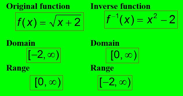
Finding the domain and range
The domain and range swap for inverse functions
Composition of f and f-1
f(f-1(x)) = f-1(f(x)) = x
If both functions, when composed with each other, cancel out, then they are inverses of each other
2.9 - Logarithmic Expressions
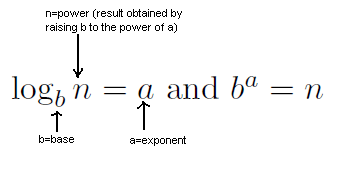
A logarithm is a way to find an unknown power using the base and a number
Ex.
log2(64) = 6 | 26 = 64
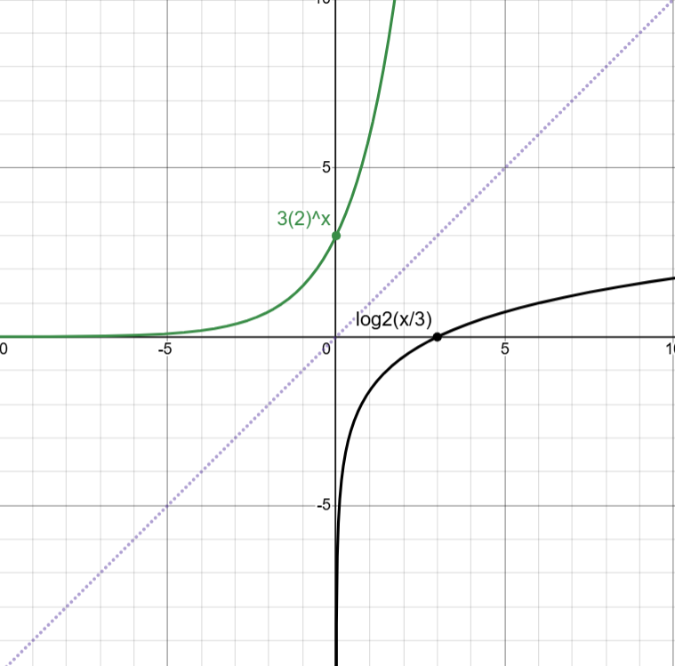
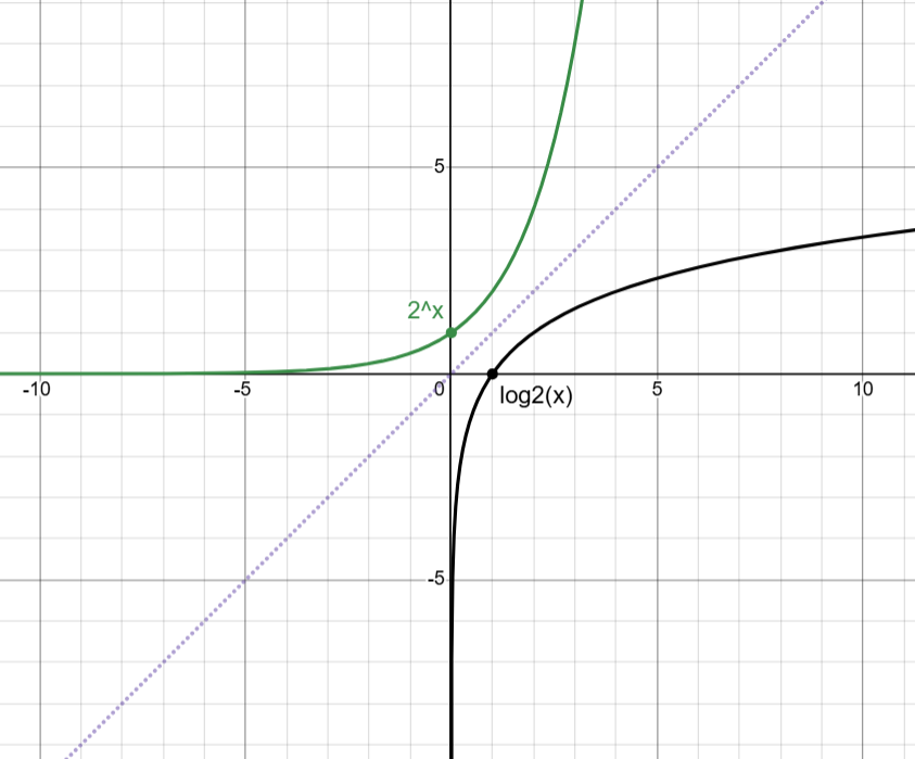
2.10 - Inverses of Exponential Functions
The inverse of an exponential function can be modeled through a logarithmic function.
Exponential vs. Logarithmic
Exponential | Logarithmic |
x values will be linear (1, 2, 3, 4) | x values will change proportionally (3, 9, 27, 81) |
y values change proportionally (2, 4, 8, 16) | y values are linear (1, 2, 3, 4) |
Power Rule → 2log5(x) = log5(x2)
Raising to a log power
if a and b are the same and c = 1, then you can cancel out to get x
2log2(x) = x
You can also cancel out to get x if the bases are the same in this scenario → log2(2x) = x
Using these two, you can find if an exponential function and a logarithm function are inverses by plugging each function into each other (ex. f(g(x)) = x = g(f(x)))
2.11 - Logarithmic Functions
Logarithmic functions have inverse properties as exponential functions
Exponential
x-intercept: NA
y-intercept: (0, 1)
asymptote: y = 0
increasing: (-∞, ∞)
decreasing: NA (only when 0 < b < 1)
domain: (-∞, ∞)
range: (0, ∞)
Logarithmic
x-intercept: (0, 1)
y-intercept: NA
asymptote: x = 0
increasing: (-∞, ∞)
decreasing: NA (only when 0 < b < 1)
domain: (0, ∞)
range: (-∞, ∞)
Transformations of Logarithm Graphs
Horizontal Translations
logb(x ± h)
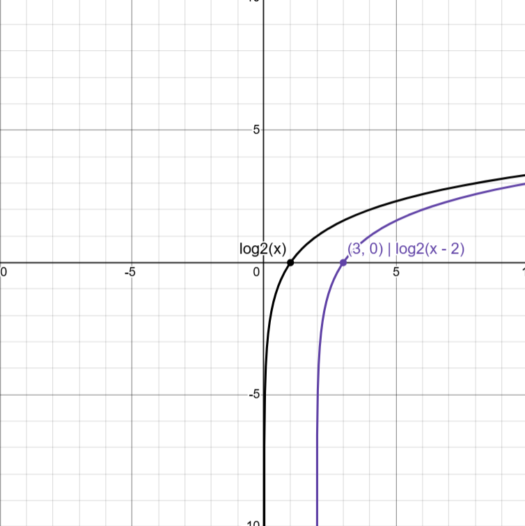
CHANGES DOMAIN
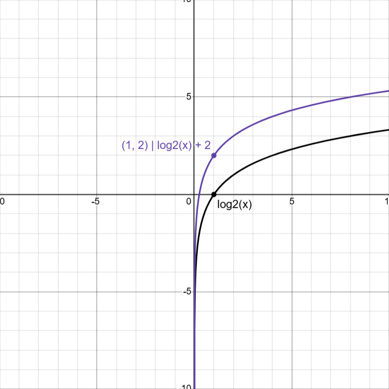
Vertical Translations
logb(x) + k
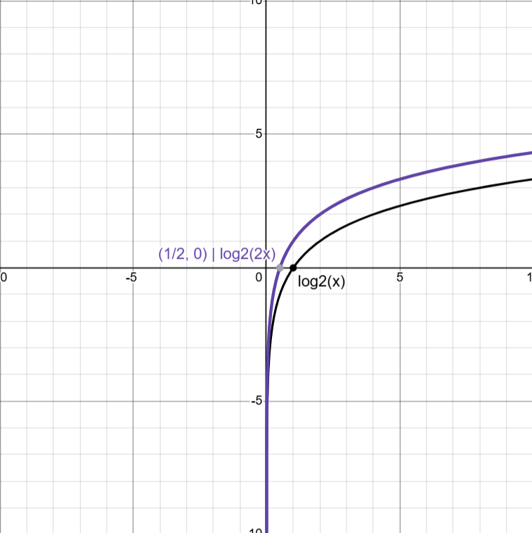
Horizontal Dilation
logb(cx)
Compresses x-values by 1/c
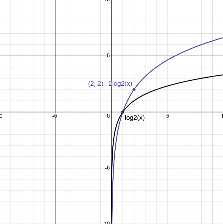
Vertical Dilation
alogb(x)
Extends y-values by a
Horizontal Reflection
logb(-x)
Reflection over y-axis
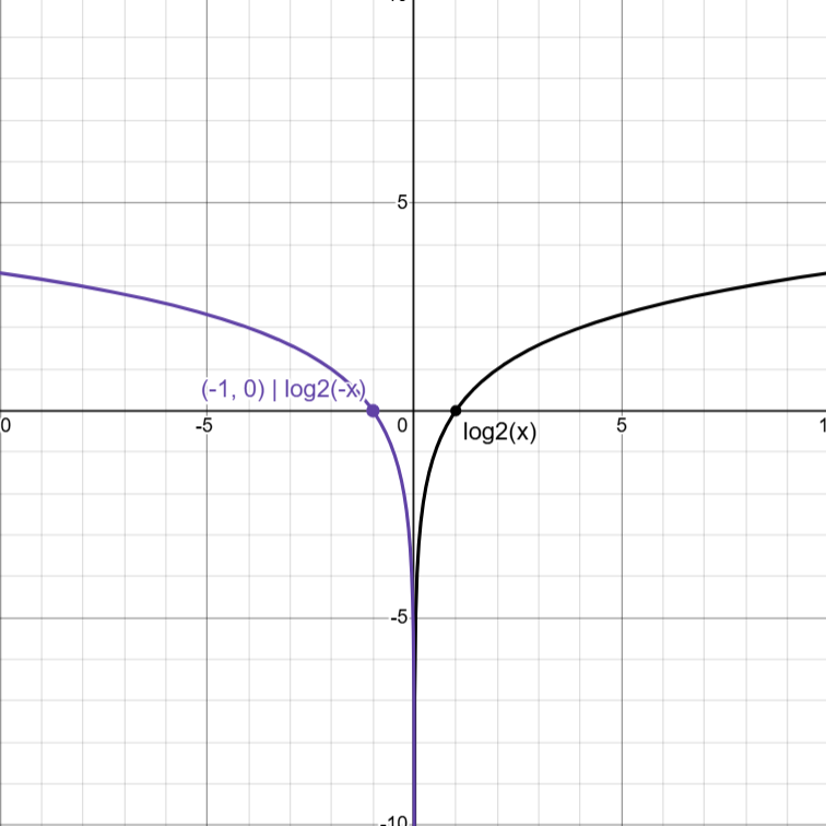
CHANGES DOMAIN
Vertical Reflection
-logb(x)
Reflection over x-axis
2.12 - Logarithmic Function Manipulation
Product Property →
Quotient Property →
Power Property →
Change Base Formula →
Equality Rule →
Finding transformations through manipulation
f(x) = log2(4x) → can be separated by product propety
f(x) = log24 + log2x → 4 can be simplified
f(x) = log2(22) + log2x → canceling out the 2s because they are the same bases
f(x) = 2 + log2x
This means that the function f(x) has a vertical translation of 2
2.13 - Exponential & Logarithmic Equations & Inequalities
Logarithmic Equations
If you have logs with the same base on each side, you can cancel them (equality rule)
log2(x + 3) = log2(5) → x + 3 = 5
You can also use logs to solve exponential equations
2(3)x - 3 = 18 → 3x - 3 = 9 → 3x - 3 = 32 → x - 3 = 2
Inequalities
First, you need to find out what restrictions there are in the inequality (making sure they are positive)
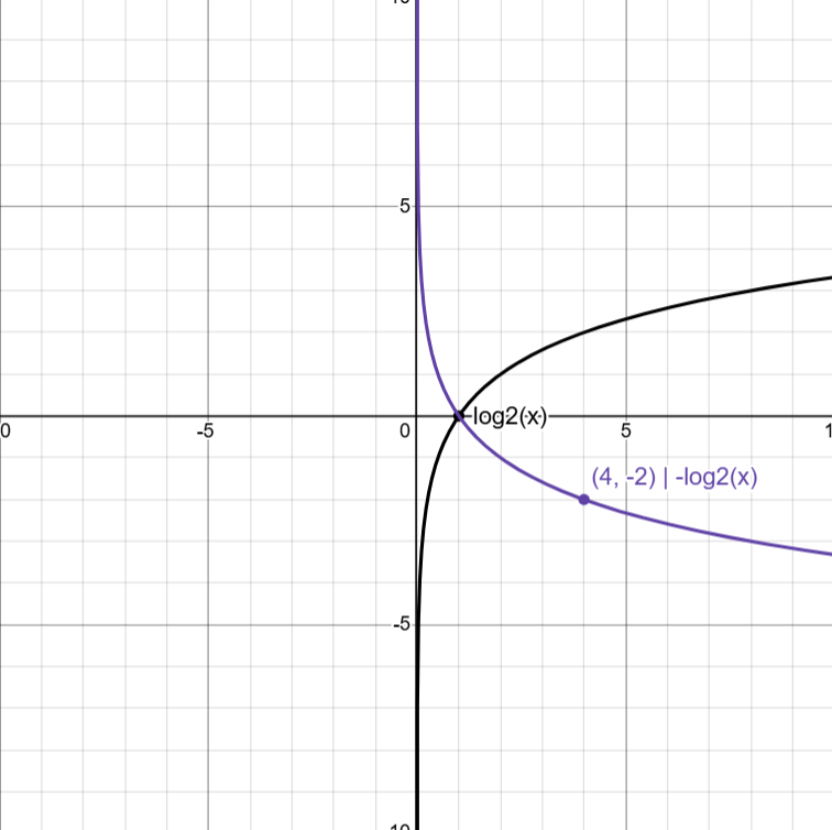
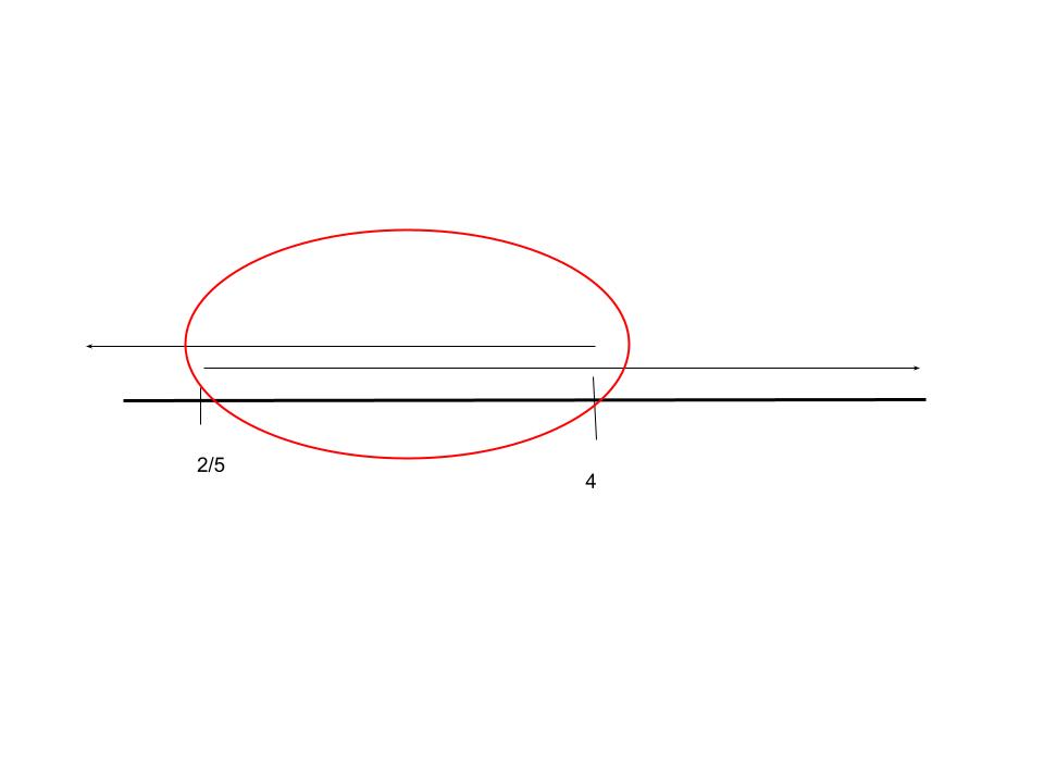
log(x + 2) + log(3) > log(5x - 2)
x + 2 > 0 → x > -2 (won’t work because it is below zero)
0 < 5x - 2 → x > 2/5
Then, you need to solve the equation
log(3x + 6) > log(5x - 2) → 3x + 6 > 5x - 2 → 6 > 2x - 2 → 8 > 2x → x < 4
Then you follow along with the restrictions and your output to get → 2/5 < x < 4
2.14 - Logarithmic Function Context and Data Modeling
Usually, when given datasets, if the x-values are proportional and the y-values are linear, then the table is logarithmic
x | 1 | 3 | 9 | 27 | 81 |
y | 3 | 5 | 7 | 9 | 11 |
You can use your calculator to use natural log regression to find the equation for these points
2.15 - Semi-Log Plots
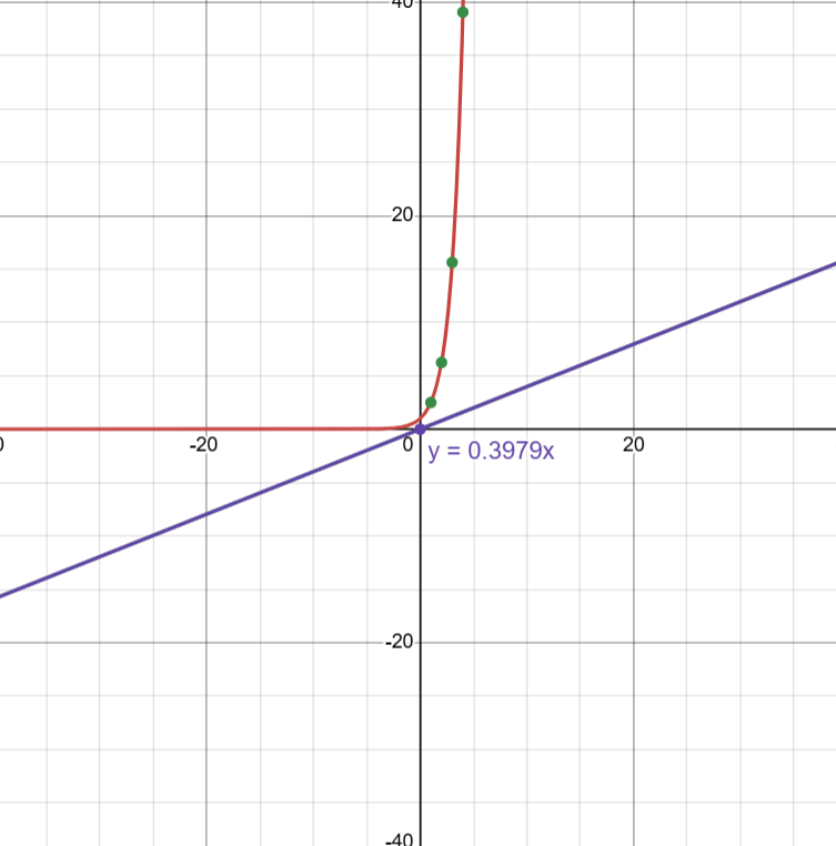
Taking these points…
x | 1 | 2 | 3 | 4 |
y | 2.5 | 6.25 | 15.625 | 39.0625 |
… you get this exponential graph…
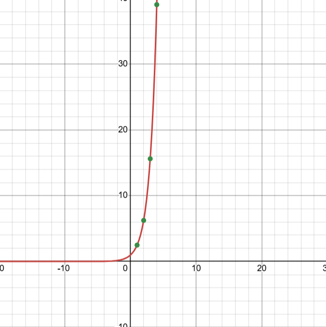
However, when you switch to a semi-log plot, the y-values appear as bases of 10 (100, 101, 102) and the graph appears linear…
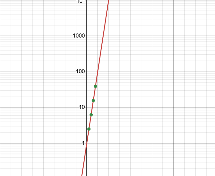
Taking the log, the equation gives this straight and linear line:
y = 1(2.5)x → log(y) = log(1) + log(2.5x) → log(y) = 0 + xlog(2.5) → y = 0.3979x
This is the same as taking the log of each of the y-values of the original function.
Unit 3
3.1 - Periodic Phenomena
A periodic function demonstrates a repeating pattern over successive equal-length intervals.
Period - the smallest change in x-values it takes for the function to repeat itself
the smallest positive value of k such that f(x + k) = f(x)
3.2A - Radians & 3.2B - Sine, Cosine, and Tangent
An angle in standard position has one ray on the x-axis (called the initial side) and another called the terminal side
Radian → a unit of angle, equal to an angle at the center of a circle whose arc is equal in length to the radius
The angle of one radian is when the angle creates an arc length on a circle that is equal to the radius of the circle
This means that and
Having a negative angle means that you go clockwise around the circle
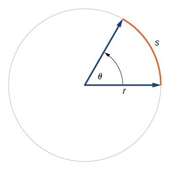
The rays of an angle that are touching the circle means that the arc is subtended by the angle
The angle (θ) in radians = Arc Length (s) / Radius (r)
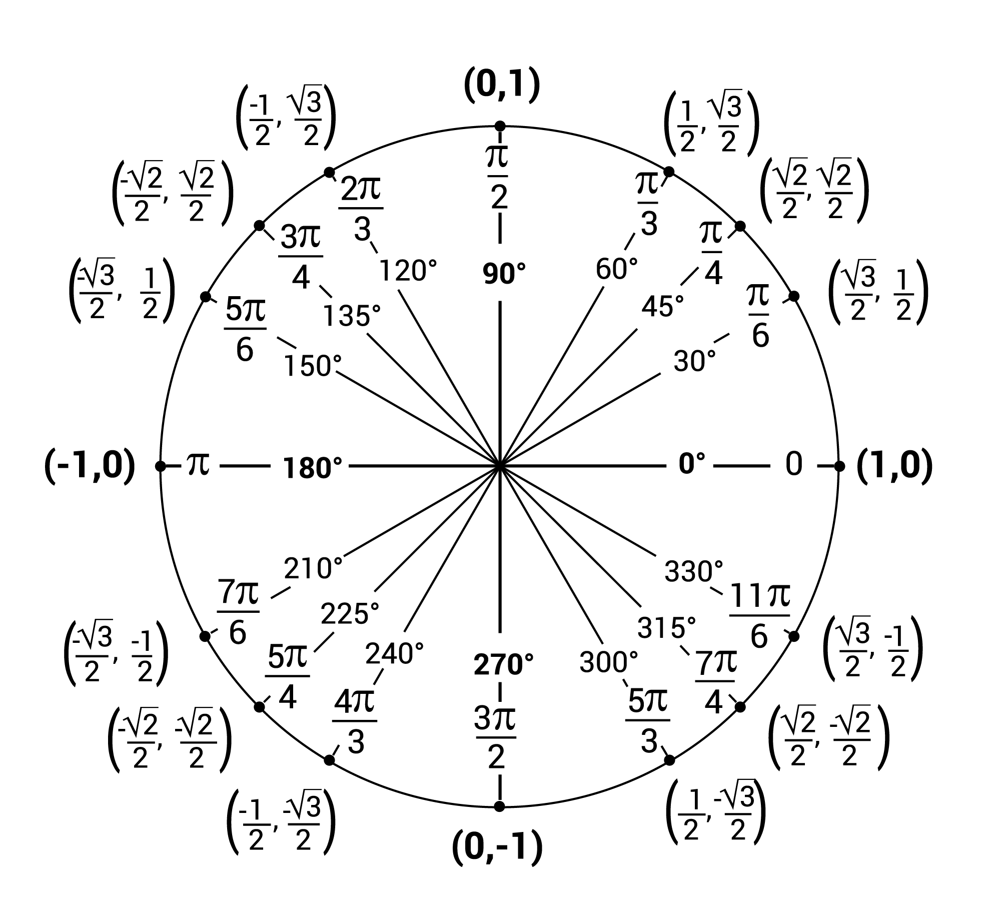
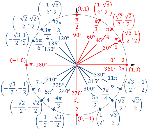
Unit Circle
The unit circle is a circle with a radius of 1
θ = s (because r = 1)
ONE REVOLUTION →
½ REVOLUTION →
¼ REVOLUTION →
REMEMBER THE UNIT CIRCLE (It will greatly help you later!)
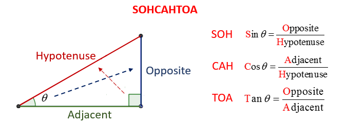
SOH-CAH-TOAH
sin(θ)
the ratio of the vertical displacement of a point (P) from the x-axis to the distance between the origin and point P
opposite / hypotenuse → y / r → y
In the unit circle,
cos(θ)
the ratio of the horizontal displacement of P from the y-axis to the distance between the origin and point P
adjacent / hypotenuse → x / r → x
In the unit circle,
tan(θ)
slope of terminal ray
An example in the unit circle →

3.3 - Sine and Cosine Function Values
Given the unit circle, when taking the cosine or sine of the radian, we can get the x and y coordinate of the point
We can also get the coordinate by using the radius and cos/sin value
Because cos(θ) = x / r → x = rcos(θ)
Because sin(θ) = y / r → y = rsin(θ)
By knowing the unit circle, you can determine where a point is as well
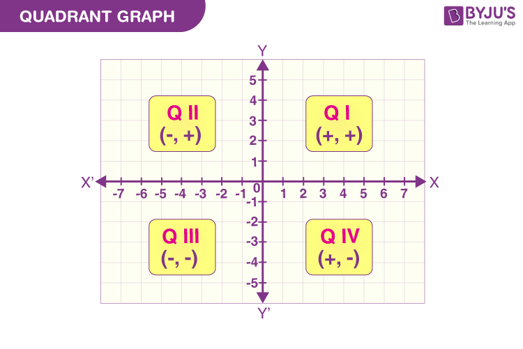
Example → (-3√3/2, -3/2)
This point has both -x and -y, so it’s in Quadrant III, meaning the points it could be is 7π/6, 5π/4, or 4π/3
The y-coordinate looks like ½, which means that the θ value is most likely 7π/6
The r value is 3 because the points have 3 multiplied onto them
3.4 - Sine and Cosine Function Graphs
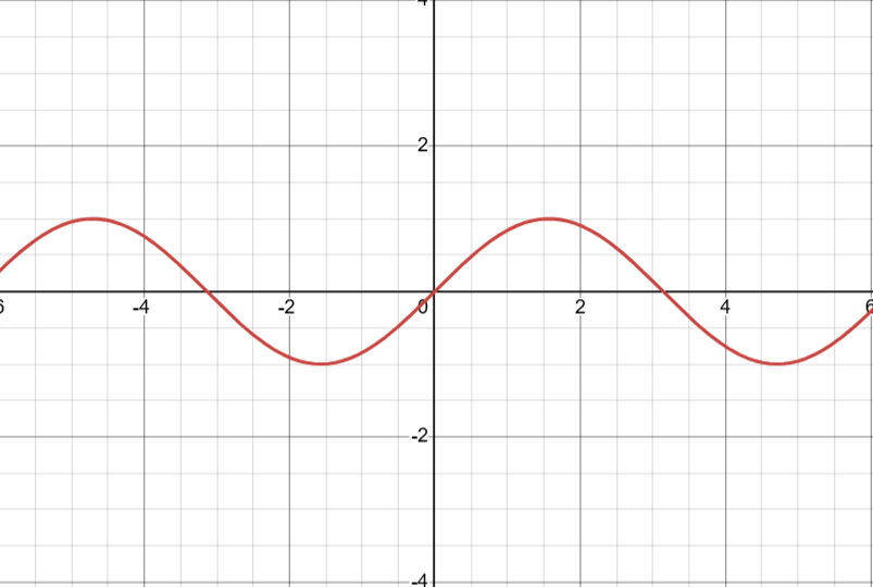
The Sine Function
y = sin(θ)
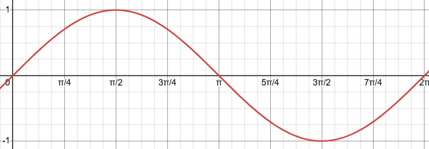
sin(θ) increases on the right side of the unit circle (0, π/2) & (3π/2, 2π)
sin(θ) decreases on the left side of the unit circle (π/2, 3π/2)
sin(θ) is concave up on the bottom side of the unit circle (π, 2π)
sin(θ) is concave down on the top side of the unit circle (0, π)
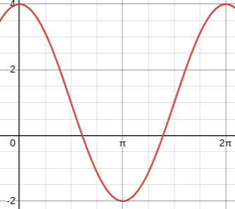
The Cosine Function
y = cos(θ)
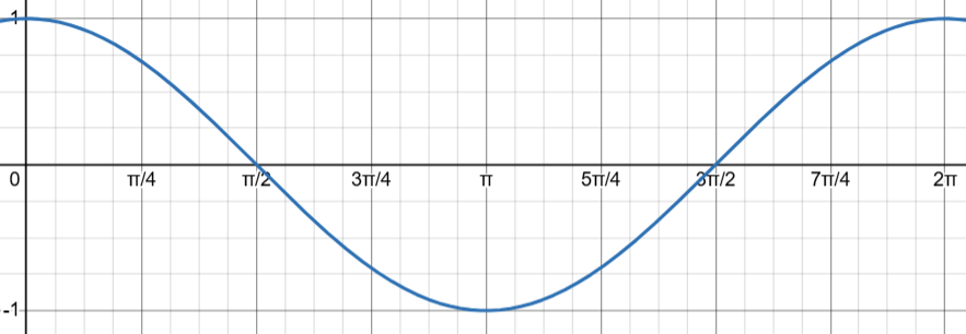
cos(θ) increases on the bottom side of the unit circle (π, 2π)
cos(θ) decreases on the top side of the unit circle (0, π)
cos(θ) is concave up on the left side of the unit circle (π/2, 3π/2)
cos(θ) is concave down on the right side of the unit circle (0, π/2) & (3π/2, 2π)
3.5 - Sinusoidal Functions
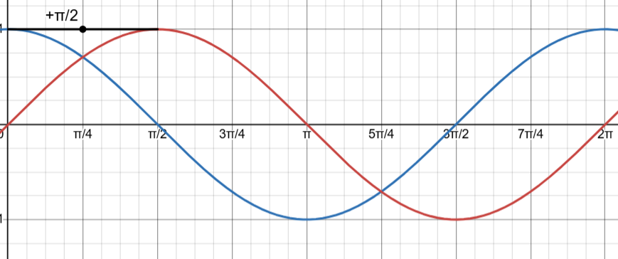
The cosine function is just the sine function -π/2 and vice versa.
Cosine is an even function and has reflective symmetry over the y-axis
Sine is an odd function and has rotational symmetry about the origin.
|
Amplitude: → half the difference between the maximum and minimum values
Midline: A horizontal line halfway between the maximum and minimum values. It is determined by finding the average of the maximum and minimum values (usually expressed as y = something)
Period (cycle): → The reciprocal of frequency. The change in θ values required for the function to complete one full cycle
Frequency: → The reciprocal of period. The number of cycles the graph completes per one radian.
3.6 - Sinusoidal Function Transformations
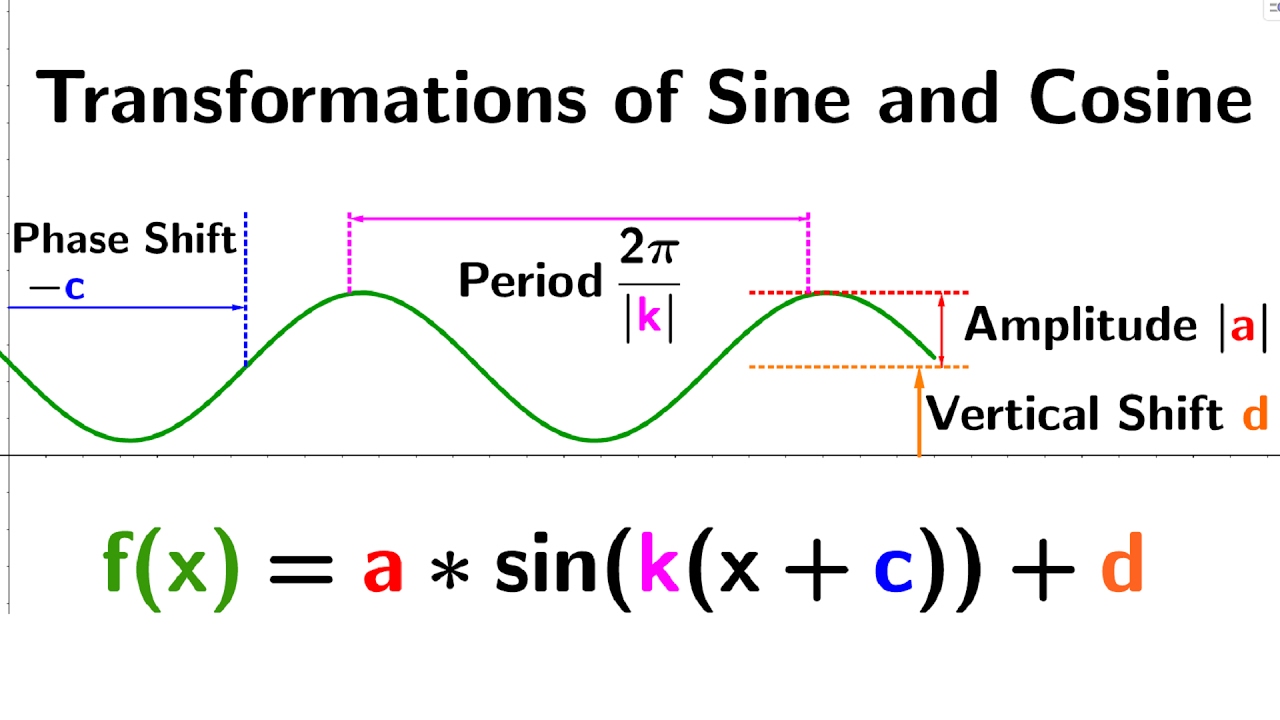
Standard Equations
Amplitude () → the amplitude / half the distance between the max and min values / ALWAYS absolute value of a / negative flips over x-axis
Midline () → A horizontal line halfway between the max and min values (also the vertical shift ±d)
Period () → The change in x values required for the function to complete one cycle (b is the horizontal stretch/shrink / negative reflects over y-axis)
Frequency () → The number of cycles the graph completes per one radian
Phase Shift () → A shift left or right (-c = right / +c = left)
Example
3.7 - Sinusoidal Function Context & Data Modeling
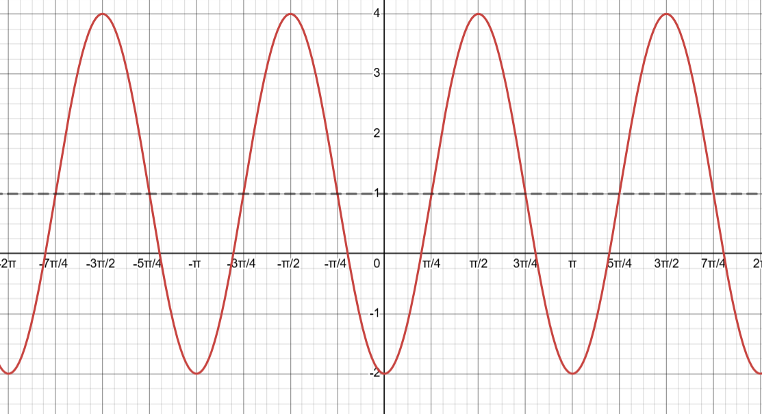
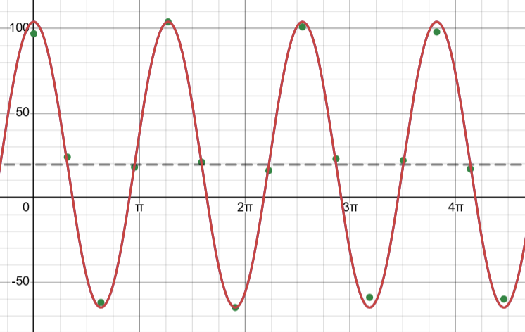
Let’s see how we can determine a sinusoidal function manually from points given to us
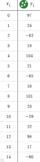
First, we need to find out where are maximum and minimum values are
Minimum → (2, -62), (6, -65), (10, -59), (14, -60)
Maximum → (0, 97), (4, 104), (8, 101), (12, 98)
We need to find the period and the frequency
For period, we just take wherever 2 maximums or 2 minimums are and subtract the x-values. We have 2 maximums at (0, 97) and (4, 104) so → 4 - 0 = 4
So, our period is 4
And thus, our frequency is
Next, we need to estimate the vertical shift / midline
This can be done by taking the highest maximum and lowest minimum and finding the average between them
Highest max → (4, 104)
Lowest min → (6, -65)
Taking the average →
Now, we find the amplitude
To find the amplitude, we just find the distance between the midline and either the highest max or the lowest min
We can use the max because it’s easier → 104 - 19.5 = 84.5
If we wanted to use the min point, we could find it as so → 19.5 - (-65) = 84.5
Using the period, we can find the b value
Finally, we need to find the phase shift
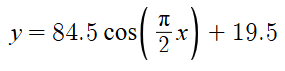
Cosine
The phase shift is easy with cosine because the maximum starts at 0 with a regular cosine function, meaning that our function is shifted by the nearest maximum to 0
In this case it is on zero, and therefore we don’t have to shift it, meaning our function looks like this →
Sine
Sine is harder because the value of 0 on sine is in between a maximum and minimum
This means we have to subtract ½ the period from the max/min closest to 0 to get the min/max
0 - 2 = -2
Next, we need to get the middle of those two points, so we just find the average (0 + -2)/2 = -1, meaning that we are shifted to the left by one which is our c value →
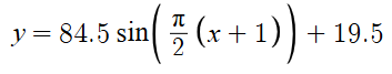
This is an estimated function, by using a calculator and using sine regression, you can find what the calculator estimated
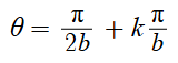
3.8 - The Tangent Function
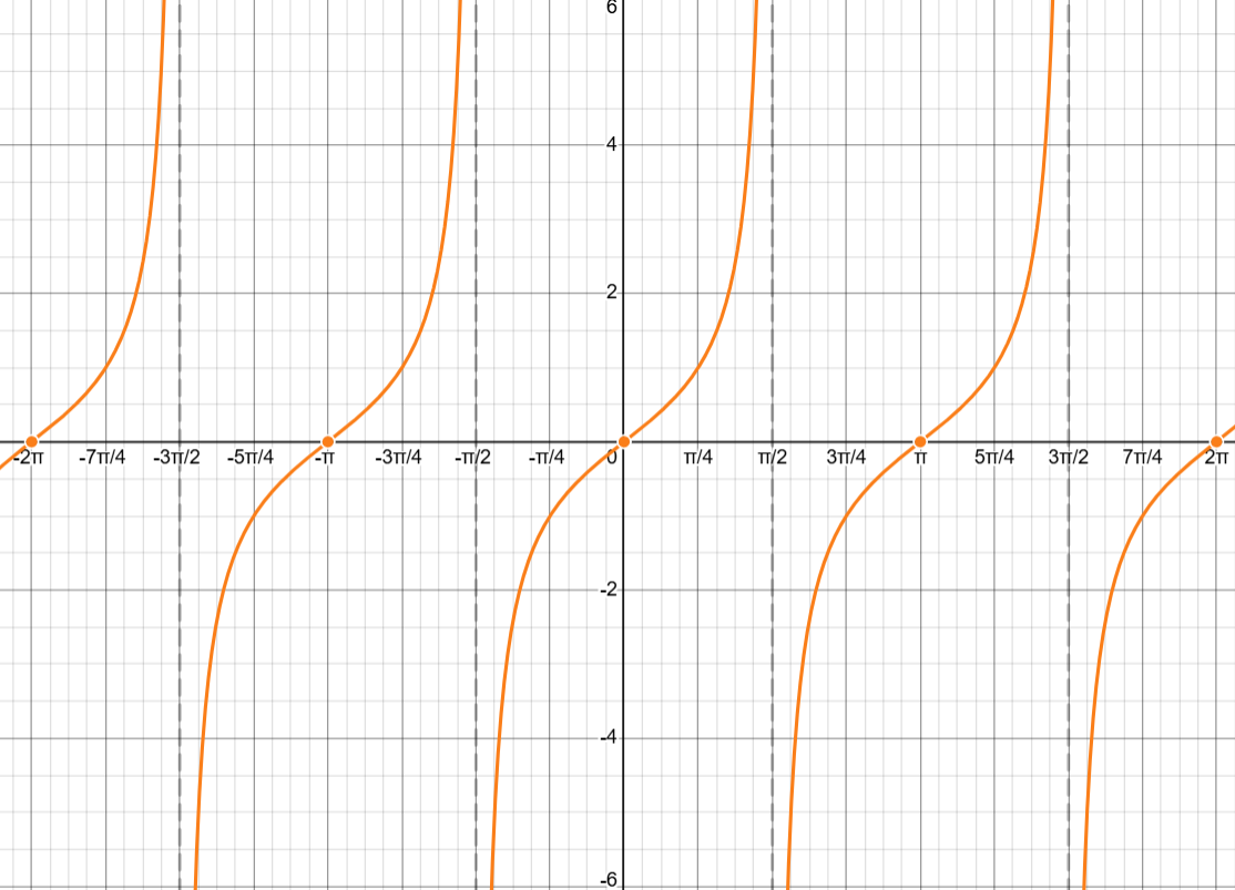
The tan(x) function gives the slope of the terminal ray
It is equal to y/x or sin(x)/cos(x) as long as cos(x) ≠ 0
Example of Point on tan(x)an(x)
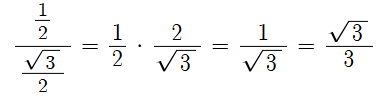
If you had tan(π/6) you just divide the sin(π/6) by cos(π/6)
sin(π/6) = 1/2
cos(π/6) = √3/2
Properties of tan(x)
The slope starts at 0
The slope gets larger until it approaches
At θ = π/2, the slope is undefined
Then the slope is infinitely negative but starts to grow towards zero
Then at π, the slope is zero again
The values of tan(x) are the same in Quadrants I & III
The values of tan(x) are the same in Quadrants II & IV
Every ½ revolution of the circle, the tangent function repeats
The period of tan(x) =
Vertical Asymptotes
For the graph tan(x), there is a vertical asymptote every →
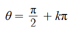
You start at and go for k periods, where k is an integer
For the graph of tan(bx), the period is π/|b|
A vertical asymptote appears every →
Where k is any integer
Transformations of Tan(x)
y = a × tan(b(x + c)) + d
a → creates a vertical dilation by the factor of |a|; If a < 0, then reflect over x-axis
b → creates a horizontal dilation and changes the period by a factor of |1/b|; If b < 0, reflect over y-axis
By either widening (0 < b < 1) or shortening (b > 1) the vertical asymptotes around each line, you can find how wide it is
c → creates a horizontal shift by -c units
d → creates a vertical shift by d units
Example
y = 2tan(1/2(x - π)) - 2
3.9 - Inverse Trigonometric Functions
Let’s say you needed to find an angle x
Using the inverse sine function, you can get rid of the sine and find the x-value
REMEMBER → the inverse of a function is just switching the x and y values. When we do this for arcsin and arccos, we cannot have two values overlapping (vertical line test), so we have a restricted range
Inverse Sine / sin-1(x) / arcsin(x)
Domain: [-1, 1]
Range:
Output values are only between side of unit circle)
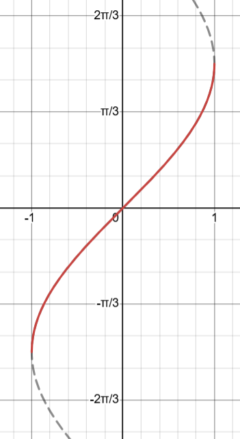
Inverse Cosine / cos-1(x) / arccos(x)
Domain: [-1, 1]
Range:
Output values are only between (top half of unit circle)
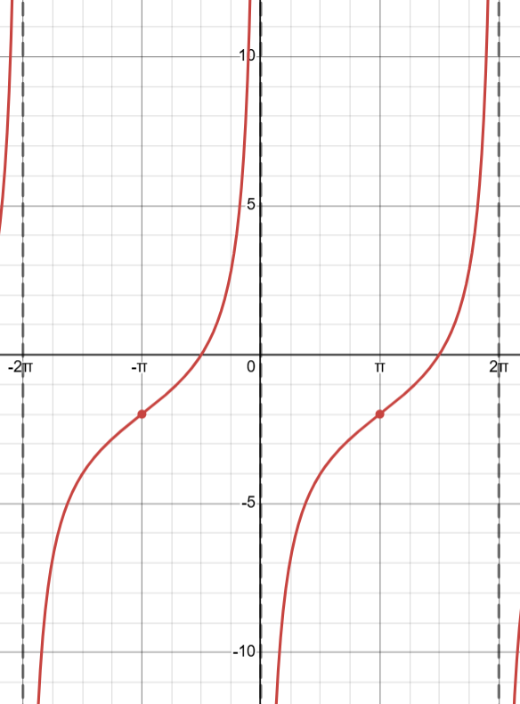
Inverse Tangent / tan-1(x) / arctan(x)
Domain:
Range:
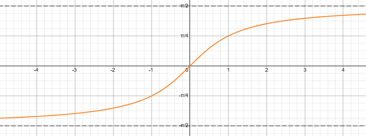
Output values are only between (right side of unit circle excluding π/2)
Finding Inverse Function
Example →
We find it like any other inverse equation
Domain & Range of f(x)
Domain →
We can find the range of f(x) normally (amplitude of 2 and midline of 1)
Range →
Swap the domain and range for
Domain →
Range →
3.10 - Trig Equations & Inequalities
Solving Trigonometric Equations
Restricted Domain (0 ≤ x ≤ 2π)
Exact Values
We can find exact values using the unit circle
Example equation →
First, we get the sin by itself
Our answer will be in values where
If we know one, for sine, the answer will be across from it → answers are also in our restricted domain, so that’s it!
Approximate Values
Approximate values we can find using a calculator
Example → (think of this as )
We can factor this out to ; this gives us two equations
Our first equation is This gives us approximately -1.326, which is our of our range, but we can get the same value by adding (instead of going clockwise, we need to go fully around the circle counterclockwise to get to the same value) →
Now we have to get the other solution to
It’s helpful to plot the point on the unit circle. 4.957 would be in Quadrant IV and we can draw a line through the origin to help us see what number the other value would be
tan(x) reflects across the origin; since this is basically half a rotation (π), we just need to subtract π from our value above → 1.816
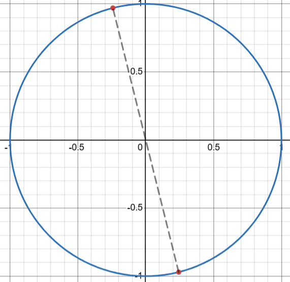
Both of these values are inside of the restricted domain, so they are are answer for the first equation → 4.957 & 1.816
Do the same thing for the other equation
All Values
Exact Values
Here, we don’t have any restricted domain, so we will format our answer differently
Example →
First, we get cos by itself →
By knowing the unit circle, we know what these values are
and the other value (for cos) can be found on the other side of the y-axis → or
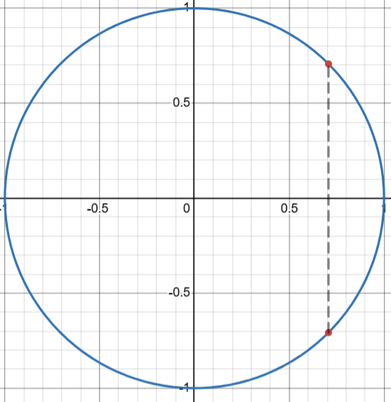
We find the other equation now →
Format the answer
Start at and every k times period (2π), we hit an answer
Approximate Values
Example →
Get everything = 0 & simplify →
Solve for each equation
(an answer every π times around the circle)
To find the other value, we know that the other value for sin will appear across from it, meaning that we can add or subtract π to get the other value)
π - 0.34 = 2.81
2.81 + 2πk where k is any integer
Solving Trigonometric Inequalities
Restricted Domain w Exact Values (0 ≤ x ≤ 2π)
Equation →
Solve like normal →
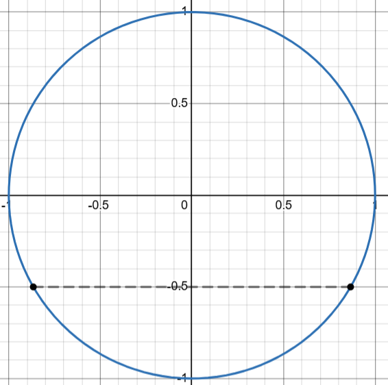
Using the unit circle, find out the two answers
Determine < or >
Because this equation is <, it would include everything to the left between the radians 2π/3 and 4π/3
Therefore, our answer is
All Exact Values
Equation →
Solve like normal, however, when taking the , don’t divide by 2
Cos equals zero at angles and
Because we hit an answer every π periods, our answer would be π/2 + πk where k is any integer
However, we divide the entire answer by the two afterwards →
3.11 - Secant, Cosecant, Cotangent Functions
Reciprocal Trig Functions
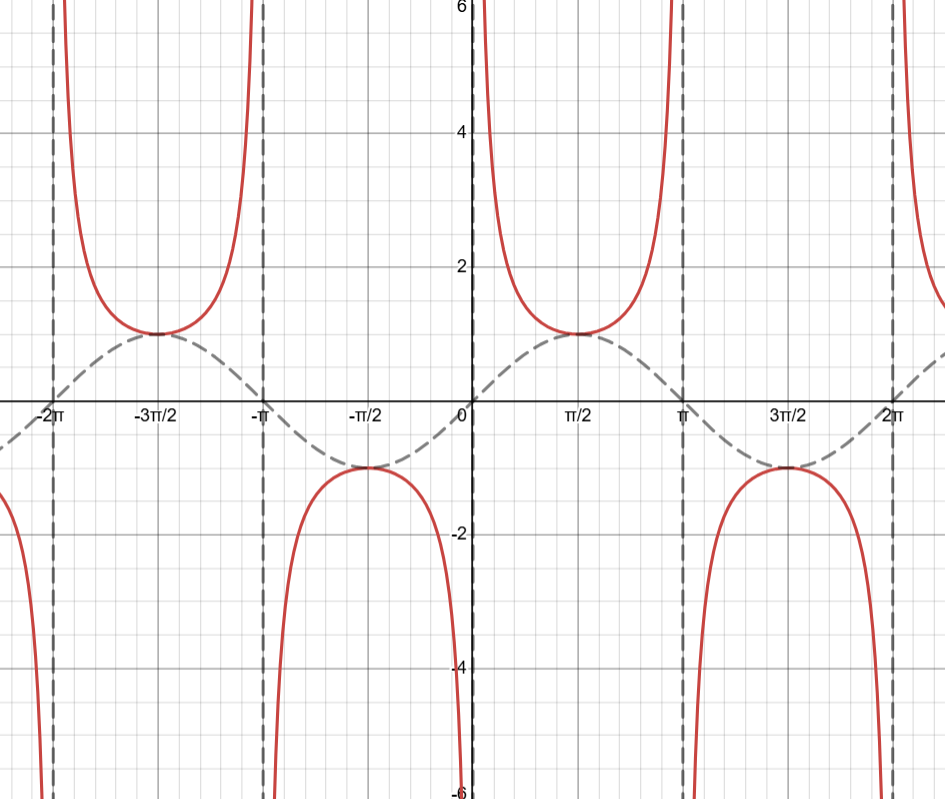
Cosecant / csc(x) / 1/sin(x)
Cosecant is or
When drawing out the sin function csc(x) has maximums and minimums at the maximums and minimums of sin(x)
csc(x) also has vertical asymptotes where sin(x) has zeros → 0 + πk where k is any integer
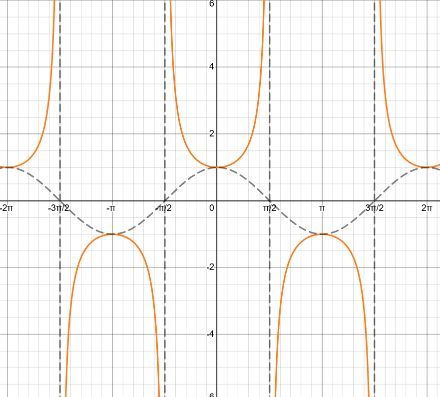
Secant / sec(x) / 1/cos(x)
Secant or sec(x) is
Sec(x) is like csc(x) where it has a max/min where cos(x) has a min/max
Sec(x) has vertical asymptotes where cos(x) has zeros → π/2 + πk where k is any integer
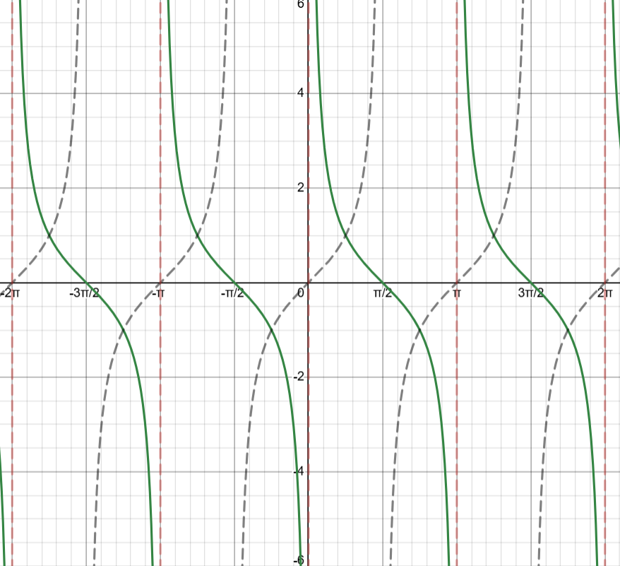
Cotangent / cot(x) / 1/tan(x) / cos(x)/sin(x)
Cot(x) is
Cot(x) has zeros where cos(x) has zeros
Cot(x) has vertical asymptotes where sin(x) has zeros → 0 + πk where k is any integer
3.12 - Equivalent Representations of Trig Functions
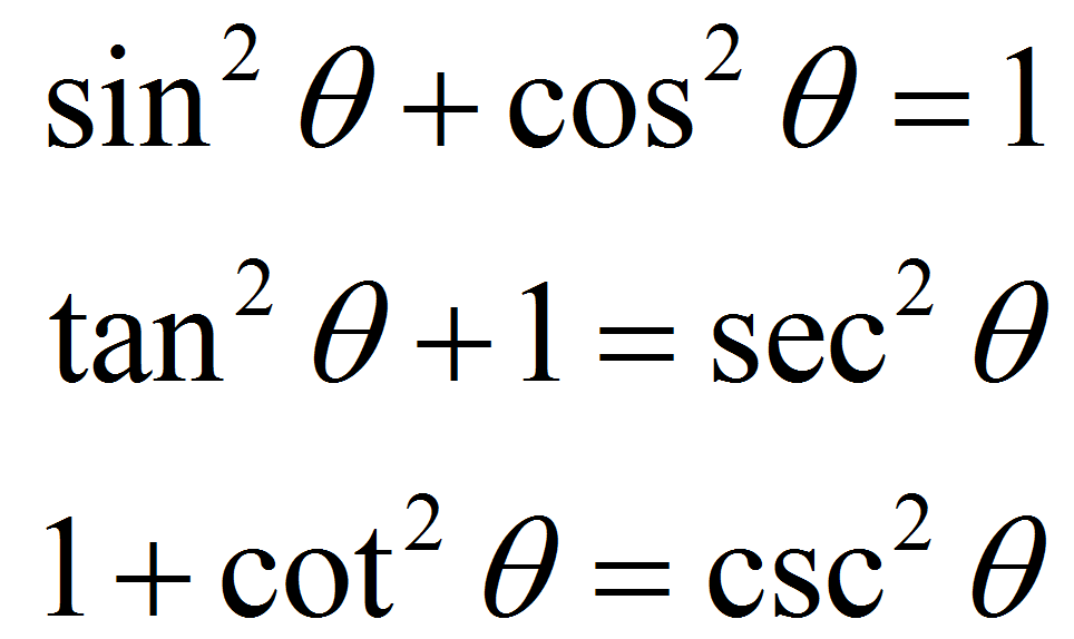
Pythagorean Identities
Our first Pythagorean identity is sin² + cos² = 1
We can also get sin² = 1 - cos²
We can also get cos² = 1 - sin²
By dividing by sin and cos, we can get our other identities
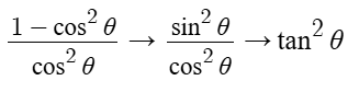
sin²/sin² + cos²/sin² = 1/sin² → 1 + cot² = csc² → cot² = csc² - 1
sin²/cos² + cos²/cos² = 1/cos² → tan² + 1 = sec² → tan² = sec² - 1
We can use these identities to simplify equations such as:
Solving Equations
Given the equation 1 = sec²x + tanx, and we need to solve for x for values 0 ≤ x ≤ 2π
By shifting everything to one side we get sec² - 1 + tan = 0
Knowing our identities, we simplify it down to → tan² + tan = 0
We cans simplify further and get two equations → tan(tan + 1) = 0
Now, we solve as we have been
tan-1(0) = 0, π
tan-1(-1) = 3π/4, 7π/4
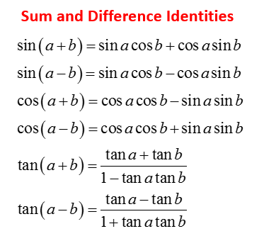
Sum/Difference Identities
The sum and difference identities look confusing, but they are easy!
Helpful Tricks
a and b, no matter the function, will be in the same place
sin keeps the same sign
cos always has cos with cos and sin with sin (coscos - sinsin)
sin has mismatched functions (sincos + cossin)
Finding Values/Simplifying Using Sum/Difference Identities
Let’s say we’re given the equation →
Use the sin identitiy →
Using the unit circle, we can get these values →
We can now multiply across →
Because they have the same denominator, we can add them together, but make sure you know how to add radicals →
To simplify, use the same process; for example, if you have → sin(x - π/6)
Use your identity → sin(x)cos(π/6) - cos(x)sin(π/6)
Then we get the equation → (√3/2)sin(x) - (1/2)cos(x)
Double Angle Identities
Double Angle Identities can be found using the sum/difference identities because f(2x) = f(x + x)
We can find them like so
sin(2a) → sin(a + a) → sin(a)cos(a) + cos(a)sin(a) → 2sin(a)cos(a)
Cosine has 3 optional values
Sine & Cosine
cos(2a) → cos(a + a) → cos(a)cos(a) - sin(a)sin(a) → cos²a - sin²a
Just Cosine
Using the Pythagorean Identities, we can swap out -sin² as cos² - 1
cos²a + cos²a - 1 → 2cos²a - 1
Just Sine
We can also swap out cos²a with 1 - sin²
1 - sin² - sin² → 1 - 2sin²a
Solving Equations
Given the equation 3cos(2x) = 2cos²x we can use our identities to solve
Because we have only cos, it’d be easier to use the cos double identity → 3(2cos²x - 1) = 2cos²x
Distribute the 3 → 6cos² - 3 = 2cos²
Set the equation = 0 → 4cos² - 3 = 0
Solve as normal!
cos-1(+√3/2) = π/2, 3π/2
cos-1(-√3/2) = π/6 , 5π/6
3.13 - Trigonometry & Polar Coordinates
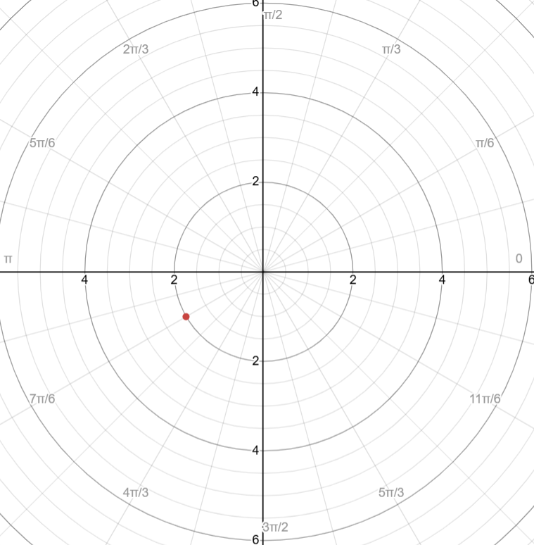
Polar Graph → a graph of concentric circles of varying radius (r) where the origin is the pole
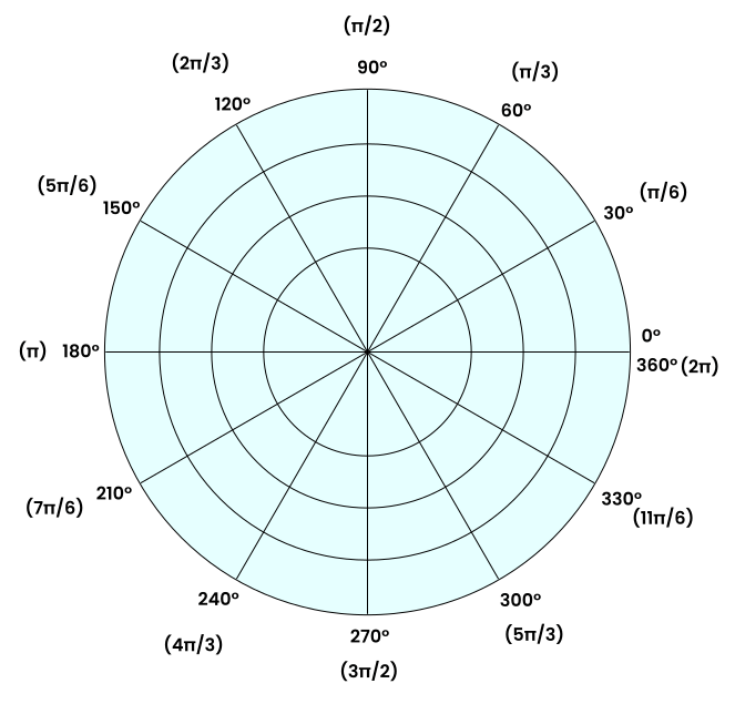
A coordinate on the polar coordinate system is (r, θ) where r is the radius (each concentric circle, counting out from the pole) and θ is the angle around the circle
When plotting points, it helps to go to the angle first and then count out to the radius
If r is negative, then you start from the origin/pole and count backwards on the angle line
For example, if you had (-2, π/6), you’d start from the origin and, on the line of π/6, count out 2 rings on the line of 7π/6
If θ is negative, then you go clockwise around the circle
Because of this, this means we can get 4 different ways to plot a point on the polar graph:
(2, 7π/6)
(-2, π/6)
(2, -5π/6)
(-2, -11π/6)
Conversions
Polar → Rectangular
This is the easier of the transformations
x = r × cos(θ)
y = r × sin(θ)
Rectangular → Polar
We can use the identities to find r (x² + y² = r²)
Because tan(θ) = y/x, we can get the angle from both points by taking the inverse
Make sure to check for boundaries and to make sure that the value in where the actual coordinate is because arctan gives 2 values
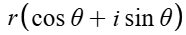
Imaginary/Complex Numbers (a + bi)
Complex Numbers consist of a real part (a) and an imaginary part (bi)

Conversions
The polar form looks like this →
Rectangular Complex → Polar Complex
This is similar to the other conversions. However, make sure that when you take the theta value, that the value would be in the actual place the coordinate is (because tan-1 has 2 values)
Example
Polar Complex → Rectangular Complex
This is also similar to the other conversion
a = r × cos(θ)
b = r × sin(θ)
Example
3.14 - Polar Function Graphs
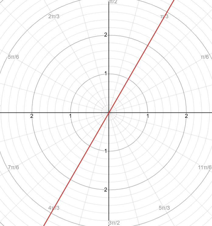
Lines
Lines are when θ = something like π/3
Circles
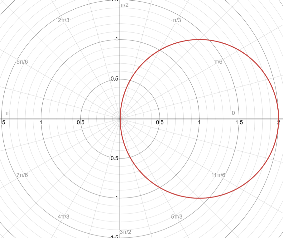
Circles are when r = a × (cos(θ) or sin(θ))
a is the maximum r values
Cosine
Example of r = 2cos(θ)
Cycle: [0, π]
Positive: open right
Negative: open left
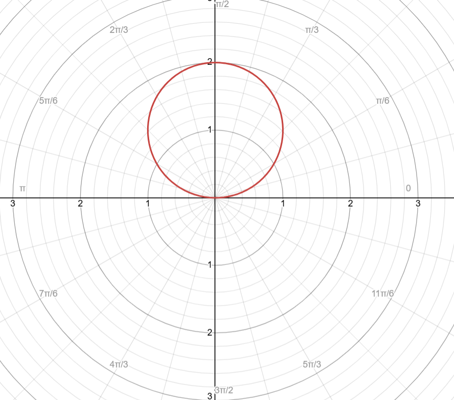
Sine
Example = r = 2sin(θ)
Cycle: [0, π]
Positive: open above
Negative: open below
Roses
Cosine → petal on x-axis
Sine → no petals on x-axis
r = a × cos/sin(nθ)
a is the max distance from the pole
n is even → 2n petals
n is odd → n petals
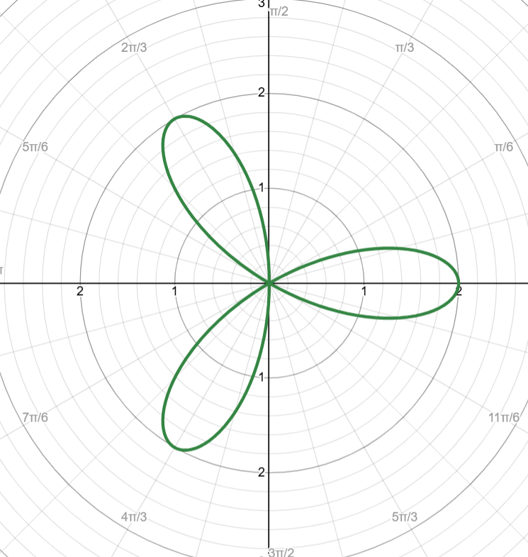
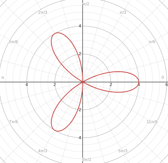
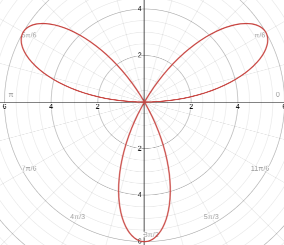
Odd n Cosine
Example → r = 2cos(3θ)
# of petals: 3
Cycle: [0, π]
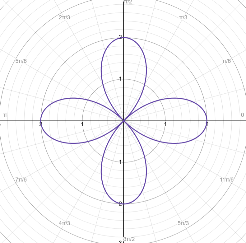
Even n Cosine
Example → r = 2cos(2θ)
# of petals: 4
Cycle: [0, 2π] (2n petals means that the cycle is double too)
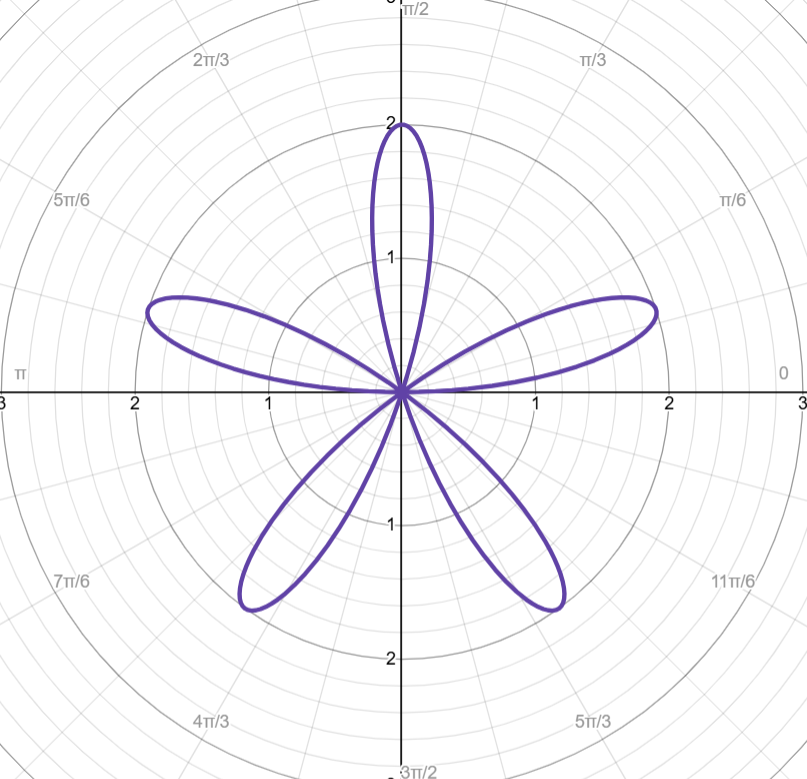
Odd n Sine
Example → r = 2sin(5θ)
# of petals: 5
Cycle: [0, π]
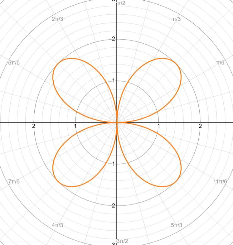
Even n Sine
Example → r = 2sin(2θ)
# of petals: 4
Cycle: [0, 2π]
Find Endpoints with Restricted Domain
For example, given the equation: r = 4cos(3θ), what are the endpoints of π/6 ≤ θ ≤ π/3
The graph would look like this
We then input both π/6 and π/3 into the equation to get our endpoints
r = 4cos(3(π/6)) → r = 4cos(π/2) = 0 → (r, θ) = (0, π/6)
r = 4cos(3(π/3)) → r = 4cos(π) = -4 →(r, θ) = (-4, π/3)
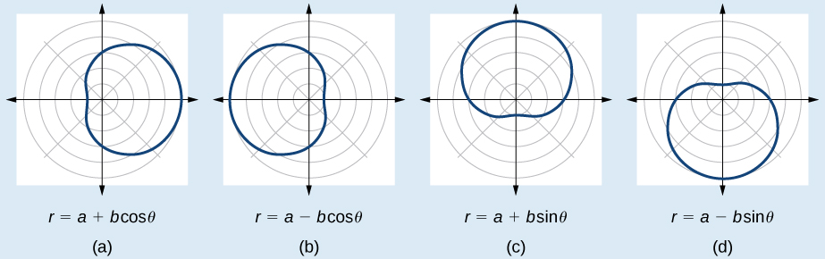
Limaçon
r = a ± bcos(θ)
r = a ± bsin(θ)
a + b → gives you the max radius
a - b → gives you the max radius in opposite direction
a > 0 and b > 0
Different ways limacons can appear based on cos/sin and + or -
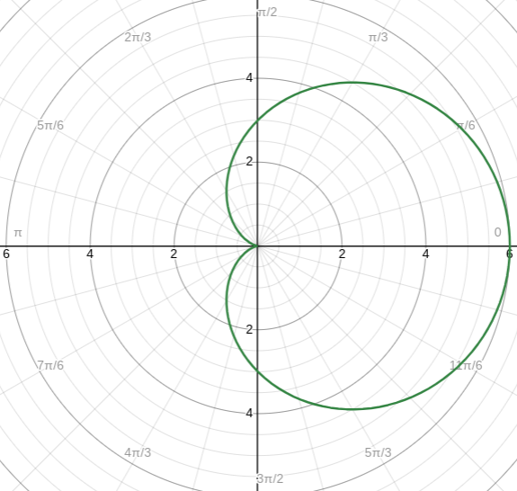
Cardioids (a = b)
Example → r = 3 + 3cos(θ)
Max r → 3 + 3 = 6
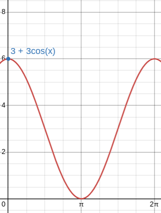
Cardioids look like hearts
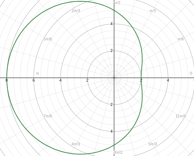
Dimpled Cardioid (a > b | 1 < a/b < 2)
Example → r = 5 - 3cos(θ)
Max r → 5 + 3 = 8
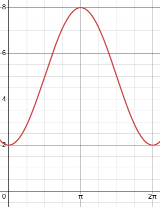
Dimples/Convex Cardioids look like their name, they have a small dent or they appear flatter on one side
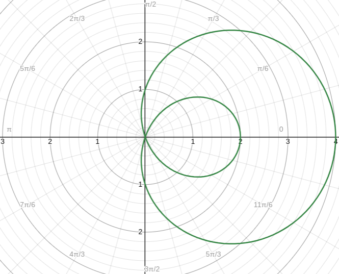
Inner Loop Limacon (a < b)
Example → 1 + 3cos(θ)
Max r → 1 + 3 = 4
Like the name, they have an inner loop
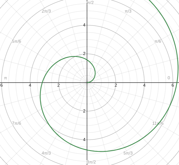
Archimedes’ Spiral
where r = θ and θ is greater than 0
3.15 - Rates of Change in Polar Functions
The Rate of Change of r
Given the equation r = 6sin(3θ), we get this graph
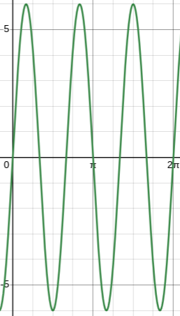
On the intervals
(0, π/6) → r is positive & increasing
(π/6, π/3) → r is positive & decreasing
(π/3, π/2) → r is negative & decreasing
(π/2, 2π/3) → r is negative & increasing
The polar version of this graph looks like this
the rate of change is measured by the distance from the pole
r is positive | r is negative | |
r = f(θ) is increasing | distance is increasing (going farther) | distance is decreasing (closer) |
r = f(θ) is decreasing | distance is decreasing (closer) | distance is increasing (going farther) |
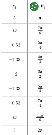
Example
Equation → r = f(θ) = 3 + 5sin(θ) on the interval π ≤ θ ≤ 2π
Here is the data table →
Interval(s) where f is increasing
r is increasing from -2 to 3 so → (3π/2, 2π)
Interval(s) where f is decreasing
r is decreasing from 3 to -2 so → (π, 3π/2)
Is there any relative extrema?
Yes, at least one because f changes from decreasing to increasing
Is the distance between r/f(θ) and the pole is increasing/decreasing on the interval 5π/4 ≤ θ ≤ 3π/2
r is negative and r is decreasing → distance is increasing from the pole
What is the AROC of f between 3π/2 and 7π/4
r2 - r1 / θ2 - θ1
-2 - (-0.53) / 3π/2 - 7π/4 = 1.871 units per radian
What interval(s) must r = 0
When it changes from + → - or - → +
(7π/6, 5π/4) & (7π/4, 11π/6)
Using the aroc above, what is the estimated value of 5π/3?
Use point-slope formula and taking a value close to 5π/3:
r1 - (-2) = 1.871(θ1 - 3π/2)
f(5π//3) = 1.871(5π/3 - 3π/2) - 2 = -1.02
Good Luck on the AP Precalculus Exam!