Getting Started with Images

1. Import Libraries:

import cv2
import numpy as np
import matplotlib.pyplot as plt
%matplotlib inline
from IPython.display import Image

2. Reading images using OpenCV:

retval = cv2.imread( filename[, flags] )

imread flags:

• cv2.IMREAD_GRAYSCALE or 0: Loads image in grayscale

• cv2.IMREAD_COLOR or 1: Loads a color image. Default flag

• cv2.IMREAD_UNCHANGED or -1: Loads image as such including alpha channel

#Read image as gray scale
checkerboard_img = cv2.imread("checkerboardImage.png", 0)
print(checkerboard_img)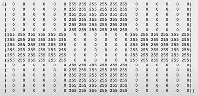

3. Displaying Images using Matplotlib:

Matplotlib uses different color maps and it is possible that the gray scale color map us not set.

#Set color map to gray scale for proper rendering
plt.imshow(checkerboard_img, cmap='gray')

4. Read and display color image:

For this example, lets use the Coca Cola logo.

#Read and display the Coca-cola logo.
Image("coca-cola-logo.png")

#Read in image
coke_img = cv2.imread("coca-cola-logo.png", 1)

print("Image size is ", coke_img.shape) # print size of image
print("Data type of image is ", coke_img.dtype) # print data-type of image

» Image size is (700, 700, 3)
» Data type of image is uint8

plt.imshow(coke_img) # display coke image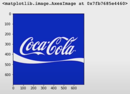

OpenCV stores images in BGR format (not RGB), this makes the color values for the RED channel and BLUE channels swapped. To display the image correctly, we have to reverse the channels of the image.

#Reverse the channels of the coke logo
coke_img_channels_reversed = coke_img[:, :, ::-1]
plt.imshow(coke_img_channels_reversed)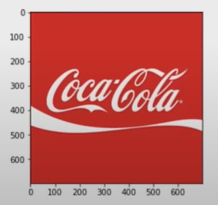

5. Splitting and Merging color channels:

• cv2.split(): Divides a multi-channel array into several single-channel arrays

• cv2.merge(): Merges several arrays to make a single multi-channel array. All the input matrices must have the same size

#Split the image into the BGR components
img_NZ_bgr = cv2.imread("New_Zealand_Lake.png", cv2.IMREAD_COLOR)
b,g,r = cv2.split(img_NZ_bgr)

#Show the individual channels
plt.figure(figsize=[20,5])
plt.subplot(141);plt.imshow(r, cmap='gray');plt.title("Red Channel");
plt.subplot(142);plt.imshow(g, cmap='gray');plt.title("Green Channel");
plt.subplot(143);plt.imshow(b, cmap='gray');plt.title("Blue Channel");

#Merge the individual channels into a BGR image
imgMerged = cv2.merge(b,g,r)

#Show the merged output
plt.subplot(144);plt.imshow(imgMerged[:,:,::-1]);plt.title("Merged Output");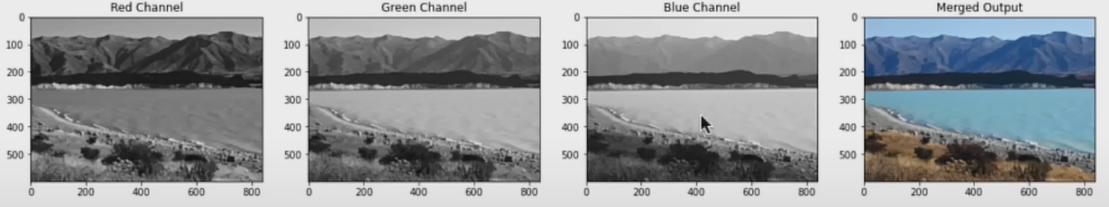

6. Converting to different Color Spaces:

A practical use for converting color spaces is changing the BGR format of OpenCV to RGB color space.

#OpenCV stores color in BGR format, unlike most other applications that store in RGB
img_NZ_rgb = cv2.cvtColor(img_NZ_bgr, cv2.COLOR_BGR2RGB)
plt.imshow(img_NZ_rgb)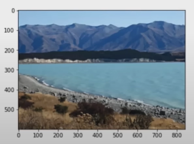

Another Color Space we can try is the HSV Color Space. (Hue, Saturation, and Value)

img_hsv = cv2.cvtColor(img_NZ_bgr, cv2.COLOR_BGR2HSV)
#Split the image into H, S, and V components
h,s,v = cv2.split(img_hsv)

#Show the channels
plt.figure(figsize=[20,5])
plt.subplot(141);plt.imshow(h, cmap='gray');plt.title("H Channel"); #Hue channel
plt.subplot(142);plt.imshow(s, cmap='gray');plt.title("S Channel"); #Saturation channel
plt.subplot(143);plt.imshow(v, cmap='gray');plt.title("V Channel"); #Value channel

#Original Image
plt.subplot(144);plt.imshow(img_NZ_rgb);plt.title("Original");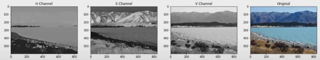

We can also modify individual channels in the HSV Color Space.

h_new = h+10
img_NZ_merged = cv2.merge((h_new,s,v))
img_NZ_rgb = cv2.cvtColor(img_NZ_merged, cv2.COLOR_HSV2RGB)

#Show modified image
plt.figure(figsize=[20,5])
plt.subplot(144);plt.imshow(img_NZ_rgb);plt.title("Modified");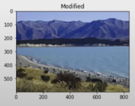

7. Saving Images:

Function syntax:

→ cv2.imwrite( filename, img[, params] )

#Save the image
cv2.imwrite("New_Zealand_Lake_SAVED.png", img_NZ_bgr)

Very similar to the cv2.imread() function of OpenCV

8. The difference between OpenCV imshow() vs Matplotlib imshow():

The main difference is how the image is displayed. Matplotlib imshow() displays the image on a graph (refer to image below) while OpenCV imshow() needs a window to display the image.

import cv2
import matplotlib.pyplot as plt

checkerboard_img = cv2.imread("checkerboard_color.png")
coke_img = cv2.imread("coca-cola-logo.png")

#Use Matplotlib imshow()
plt.imshow(checkerboard_img)
plt.title("matplotlib imshow")
plt.show()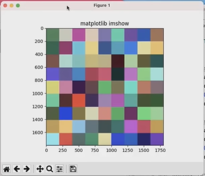

#Use OpenCV imshow(), display for 8 seconds
window1 = cv2.namedWindow("w1") #Create named window first
cv2.imshow(window1, checkerboard_img) #Argument is the window created and what to show in the window
cv2.waitkey(8000) #Almost always used in conjuction with the imshow() function
cv2.destroyWindow(window1) #Don't forget to destroy window to free space

If you look closely, you cannot press the “close” button.

#Use OpenCV imshow(), display for 8 seconds
window2 = cv2.namedWindow("w2")
cv2.imshow(window2, coke_img)
cv2.waitkey(8000)
cv2.destroyWindow(window2)

Same for the Coke image, the window will close after 8 seconds. To control how to close the window, use cv2.waitkey(0) to close on any keypress.

#Use OpenCV imshow(), display until any key is pressed
window3 = cv2.namedWindow("w3")
cv2.imshow(window3, checkerboard_img)
cv2.waitkey(0)
cv2.destroyWindow(window3)

Another implementation of cv2.waitkey(0) in a while loop:

#While loop example
window4 = cv2.namedWindow("w4")

Alive = True
while Alive:
	#While Alive is true, display until 'q' key is pressed
	cv2.imshow(window4, coke_img)
	keypress = cv2.waitkey(1)
	if keypress == ord('q'):
		Alive = False
cv2.destroyWindow(window4)

cv2.destroyAllWindows()
stop = 1

END of MODULE 1