All the mathy things in AP stats

Experimental Designs

• Completely Randomized

  

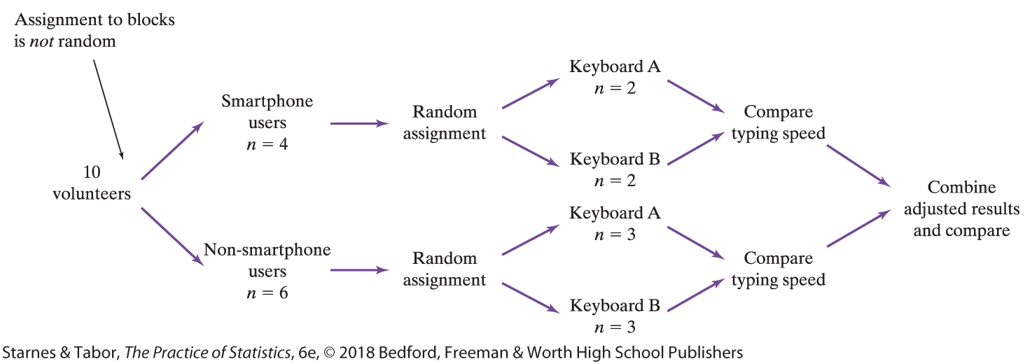
• Randomized Block

  

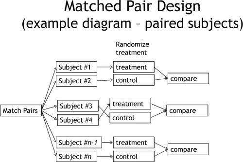
• Matched Pairs

  

  ---

Probability Models/Rules

• Two-Way Tables

  

• Venn Diagram

  

• Equally Likely Outcomes:

  P(A) = Number of outcomes in event A / Total number of outcomes in sample space

• Complement Rule: P(A^c ) = 1 - P(A)

• Addition Rule for Mutually Exclusive Events: P(A or B) = P(A) + P(B)

• General Addition Rule: P(A or B) = P(A) + P(B) - P(A n B)

• Conditional Probability: P(A | B) = P(A n B) / P(B)

• General Multiplication Rule: P(A and B) = P(A n B) = P(A) x P(B | A)

• Multiplication Rule for Independent Events: P(A and B) = P(A n B) = P(A) x P(B)

Transforming and Combining Random Variables

Continuous Random Variables: Can take any value in an interval on the number line.

E(x) = x₁p₁ + x₂p₂ + x₃p₃

σ² = (x₁ — μ₁)²p₁ + (x₂ — μ₂)²p₂ + (x₃ — μ₃)²p₃

Linear Transformations

Rule for Means: μ_a+bX = a+b(μ_x)

Rule for Variances: σ²_a+bX = b²σ²x

• x must be a constant

• adding/subtracting doesn’t change measures of variability (range, IQR, SD), or shape of the probability distribution. It does change measures of center and location (mean, median, quartiles, percentiles).

• Multiplying/dividing changes measures of center and location and measures of variability, but not the shape of the distribution.

Comparing Independent Random Variables

Where difference is D = X - Y and the sum is S = X + Y

Rules for combining means:

• μ_D = μ_{X - Y} = μ_X - μ_Y

• μ_S = μ_{X + Y} = μ_X + μ_Y

Rules for combining variances:

• σ²_D = σ²_{X - Y} = σ²_X + σ²_Y

• σ²_S = σ²_{X + Y} = σ²_X + σ²_Y

Where there is a linear transformation difference is D = bX - cY and the sum is S = bX + c

Rules for combining means:

• μ_D = μ_{bX - cY} = bμ_X - cμ_Y

• μ_S = μ_{bX + cY} = bμ_X + cμ_Y

Rules for combining variances:

• σ²_D = σ²_{bX - cY} = b²σ²_X + c²σ²_Y

• σ²_S = σ²_{bX + cY} = b²σ²_X + c²σ²_Y

Binomial Distributions (6.3)

Necessary Settings:

• Binary? - outcomes can be classified as “success” or “failure”

• Independent? - knowing the outcome of one trial doesn’t tell anything about the outcome of another trial

• Number? - the number of trials of the random process is fixed in advance

• Same Probability? - there is the same probability of success in each trial

the Binomial Coefficient - the number of ways to arrange x successes among n trials

• nCr → [Math] [Prob] [3]

• ! → [Math] [Prob] [4]

Precise Functions

• binompdf (n, p, x) → [2^nd] [Vars] [A]

Continuous Functions

• binomcdf (n, p, x) → [2^nd] [Vars] [B]

• P( x < 3 ) = p( x = 0 ) + p( x = 1 ) + p( x = 2 )

expected count of successes:

As the sample size becomes larger, the Binomial Distribution becomes more like a Normal Distribution. If the following conditions are fulfilled then the sample size is large enough to consider the distribution normal:

• 10% condition

• Large Counts Condition: at least 10 expected successes and 10 expected failures

Geometric Distributions (6.4)

If an experiment has two possible outcomes of success (p) and failure (1-p), and the trials are independent.

The probability that the first success is on trial number k:

• P(X = k) = ( 1- p)^k-1p

• P(X = k) →geometpdf → [2nd] [Vars] [F] → (prob, x-value)

• P(X ≤ k) →geometpdf → [2nd] [Vars] [G] → (prob, x-value)

Sampling Distributions

Sampling Distributions of p hat

7.2

Sampling Distributions of x bar

7.3

Confidence Intervals

use t* or z*

Confidence Intervals 1-prop

8.2

Confidence Intervals for p1-p2

8.3

Confidence Intervals for U (mew)

10

confidence interval for a difference between two means (two-samp)

10.2

confidence interval for U diff (paired)

10.2

t-interval for the slope

12.3

Significance Tests

About a Proportion - 1-prop (9.2)

One sided

S: H₀ : p = p₀

H_a : p > p₀ -or- H_a : p < p₀

P: One sided z-test for p̂

• Random: The data comes from a random sample from the population of interest.

• 10%: when sampling without replacement, n < 0.1N

• Large Counts: Both np₀ and n( 1 - p₀) are at least 10

D:

P(p < p₀) →normcdf → [Stat] [tests] [5] → (-1e99, z, 0, 1)

P(p > p₀) →normcdf → [Stat] [tests] [5] → (z, 1e99, 0, 1)

C: Because our p-value of p < a = 0.05, we reject H₀ . We have convincing evidence that…

Two sided

S: H₀ : p = p₀

H_a : p ≠ p₀

P: Two sided z-test for p̂

D: P(p ≠ p₀) →normcdf → [Stat] [tests] [5] → (-1e99, z, 0, 1)x2

interpret the p-value - “assuming H₀ is true, there is a p probability of getting a sample mean of ___ by chance alone in a random sample of n.”

Power

the probability that the test will find convincing evidence that H_a is true when H₀ is true.

interpret - “If the true proportion of population is p₀ , there is a power probability of finding convincing evidence that H_a : p < p₀ is true.”

Power increases when:

• the sample size n is larger

• the significance level a is larger

• the null and alternative parameters are further apart

About a Difference in Proportions - 2-prop (9.3)

significance test about a mean

11

significance test with a difference in means (2-samp)

11.2

significance test about U diff (paired t-test)

11.2

significance test for the slope

12.3

X² Test for Goodness of Fit (12)

12

test for homogeneity

11.2

test for independence/association

11.2