IS-LM Model and Macroeconomic Policy

Page 1 - Key concepts

• Key Concepts:

  • Output, aggregate expenditure, and the rate of interest: the IS relation

  • Money, monetary policy, and equilibrium in the money/financial system: the LM relation

  • Simultaneous equilibrium in goods and money markets

  • Monetary and fiscal policy in terms of the IS-LM model

  • Applications of the IS-LM model

Page 2 - Assumptions in the IS model and definition of IS curve

• Assumptions:

  • Given price level and money wages (fixed)

  • Unemployed resources, ensure if there is an aggregate demand there would be increase in aggregate output.

  • Autonomous components of consumption and investment negatively related to the rate of interest. e.g. in interest up autonomous goes down.

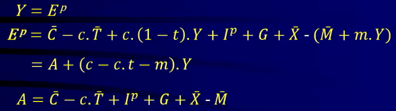
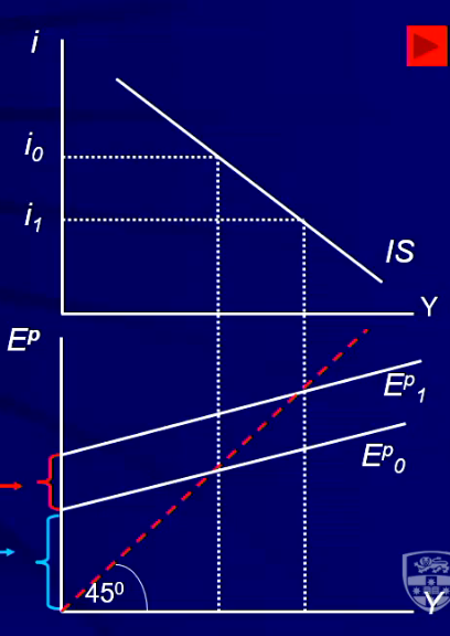
• IS Relation:

  • Combinations of interest rate (i) and output (Y) consistent with goods market equilibrium

  • Increase in autonomous demand due to a fall in interest rate leads to higher equilibrium income

The IS curve represents the relationship between interest rates and output (GDP) in the goods market, showing combinations where investment equals savings. It is derived from the equilibrium condition where total spending (consumption + investment + government spending + net exports) equals total output.

• in this case, the IS curve represents the relationship between interest rates and autonomous spending (roughly the same thing)

To derive it:

1. Start with the aggregate demand equation: ( Y = C + I + G + (X - M) ).

2. Substitute consumption and investment functions.

3. Set ( Y ) equal to aggregate demand to find the relationship between interest rates and output, resulting in the downward-sloping IS curve.

Page 3 - equilibrium condition

• Equilibrium Condition:

We are going to assume autonomous expenditure have two parts:

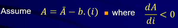
1. autonomous spending that is independent of both income and interest rate.

2. dependent of the interest rate

• Reflects an inverse relationship between output and the rate of interest

Page 4 - good market equilibrium and IS curve formation

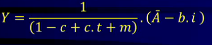
• Goods Market Equilibrium:

  • Equilibrium condition derived from the IS relation

  • Vertical intercept of the equilibrium output depends on the interest rate

    

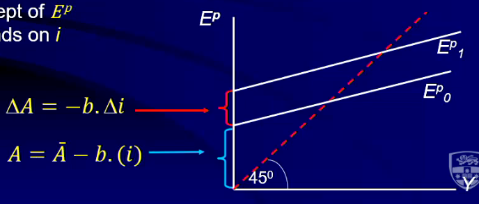
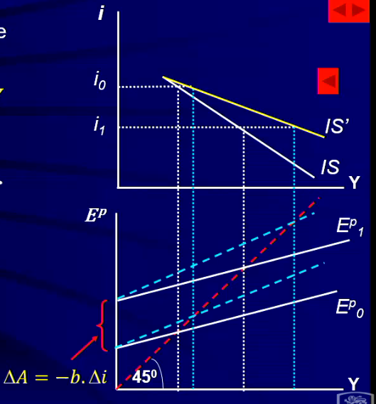
Page 5 - effect of changes in autonomous demand

• Effect of Changes in Autonomous Demand that are not affected by the rate of interest (A-bar):

  • Increase in autonomous demand (the PAE curve below) shifts the IS curve rightward and vice versa.

    

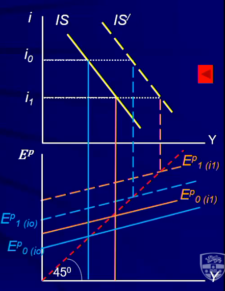
  • Repeated shifts at each level of interest rate

Page 6 - Autonomous shocks to the IS

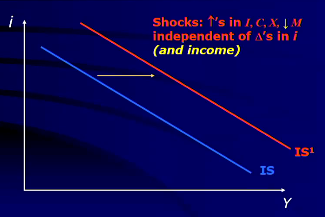
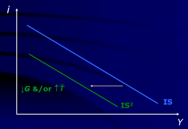
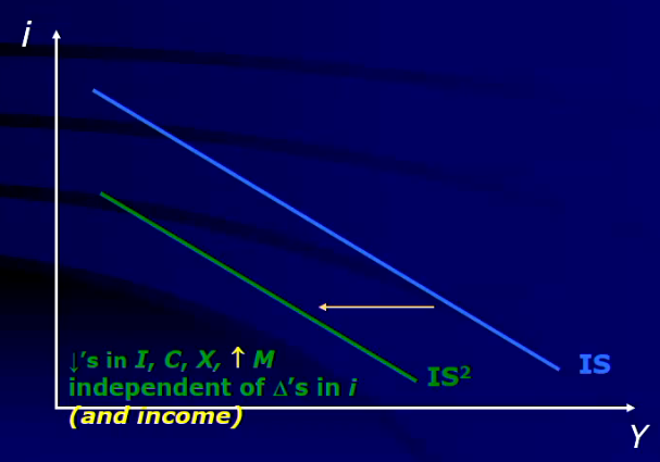
• IS Shocks:

  • Changes in investment (I), consumption (C), and exports (X) and inverse changes in import, independence of changes in income lead to shifts in the IS schedule.

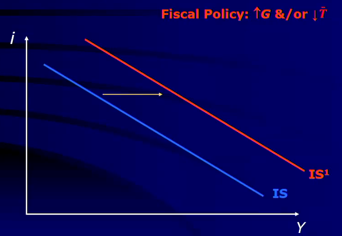
  • Fiscal policy impacts through changes in government spending (G) and exogenous tax (T-bar)

    

Page 7 - IS and multiplier relationship

• IS Curve and Multiplier:

  • we already know the multiplier from the PAE curve.

  • Larger interest elasticity of investment leads to a flatter IS curve

  • The multiplier effect is larger with higher elasticity

    

Page 8 - the LM curve derivation

To derive the LM curve, follow these steps:

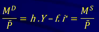
1. Money Market Equilibrium: Set the demand for money (Md) equal to the supply of money (Ms).

   [ M_d = M_s ]

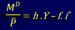
2. Money Demand Function: Typically, money demand is a function of income (Y) and the interest rate (i):

   [ M_d = L(Y, i) ]

3. Rearranging: Solve for the interest rate (i) in terms of income (Y):

   [ i = f(Y) ]

4. Graphing: Plot the relationship between income (Y) and the interest rate (i) to obtain the LM curve, which is upward sloping.

This curve represents combinations of interest rates and levels of income where the money market is in equilibrium.

• LM Relation:

  • Combinations of interest rate and output (level of income) consistent with equilibrium in the money market equilibrium

    

  • Money supply (MS) and money demand (MD) determine equilibrium

    

  • quantity of money is demand determined.

Page 9 - the IS curve and its relationship to monetary policy

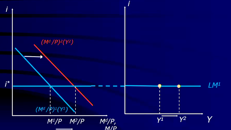
• Changes in Income via product market:

  • Shifts in money demand schedule due to changes in income

  • Horizontal LM curve when interest rate is policy-determined

    

Page 10

• Recap of Equilibrium:

  • Equilibrium in financial markets maintained by monetary policy

  • Changes in monetary policy affect the equilibrium interest rate

Page 11 - quantity vs rate-setting monetary policy, and the illustration of the LM curve

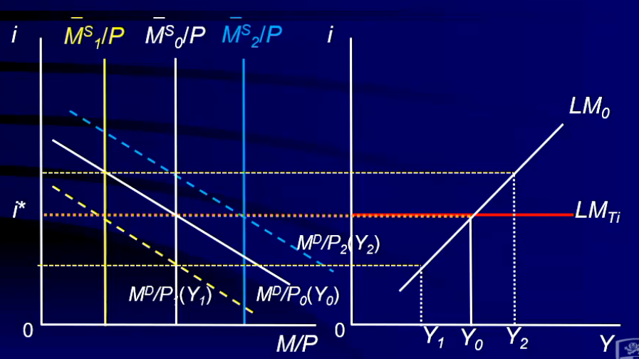
• Quantity vs. Rate-setting Monetary Policy:

  • Illustrates the relationship between money supply and interest rates

    

• if level of income increasing or decreasing, the money supply would shifts either left or right.

• if the central bank assumed an interest rate for the economy quantity of money to adapt to, the LM curve would be horizontal.

  

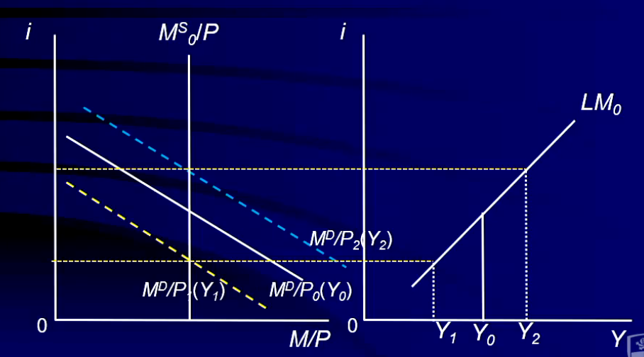
The LM curve can be horizontal or upward sloping under different conditions:

• Horizontal LM Curve: This occurs when the money supply is perfectly elastic, typically in a liquidity trap where interest rates are at or near zero. In this case, increases in money supply do not raise interest rates, leading to a flat LM curve.

• Upward Sloping LM Curve: This is the standard case where an increase in income leads to higher interest rates, reflecting the demand for money. As income rises, people want to hold more money, which increases interest rates if the money supply is fixed.

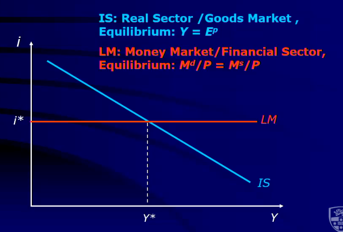
Page 12 - IS-LM equilibrium

• Macroeconomic Equilibrium:

  • Occurs at the intersection of IS and LM schedules

  • Both real income and interest rate are at equilibrium levels at which both the product market in aggregate and the money/financial market are in equilibrium

    

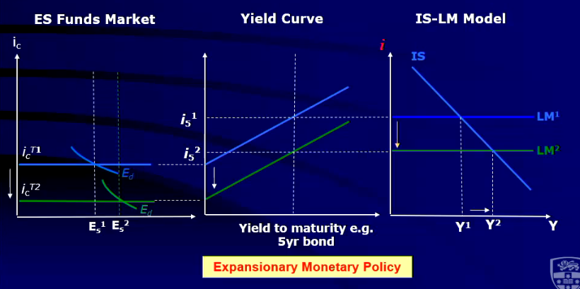
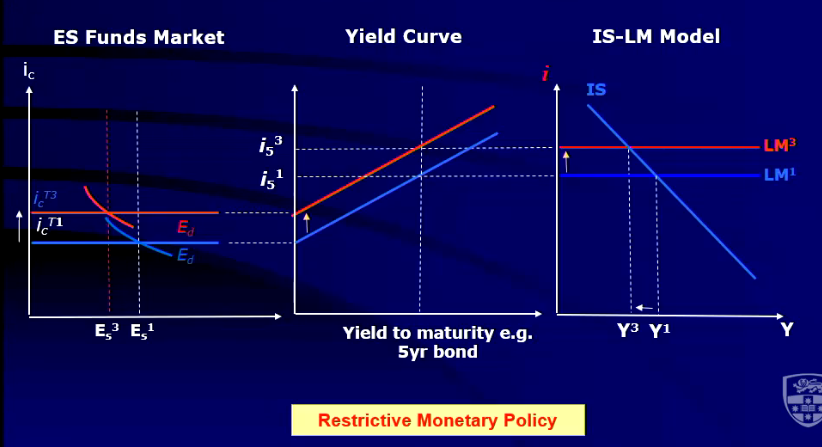
Page 14 - changes in monetary policy on the economy

• Monetary Policy Changes:

  • Changes in monetary policy shift the LM schedule

  • Expansionary vs. restrictive monetary policy effects

    

Page 15 - the effectiveness of monetary policy

• Effectiveness of Monetary Policy:

  • Depends on interest elasticity of aggregate expenditure and size of the income-expenditure multiplier

  • Flatter IS schedule indicates more effective monetary policy

So:

• a larger/smaller interest-eleasticity or multiplier = a flatter/steeper IS curve = more/less effective monetary policy

The effectiveness of monetary policy depends on the interest elasticity of aggregate expenditure and the size of the income-expenditure multiplier for the following reasons:

1. Interest Elasticity: Higher interest elasticity means that changes in interest rates significantly affect consumption and investment. If aggregate expenditure is sensitive to interest rate changes, monetary policy can effectively influence economic activity.

2. Income-Expenditure Multiplier: A larger multiplier indicates that an initial change in spending leads to a more significant overall impact on income and output. This amplifies the effects of monetary policy, making it more potent in stimulating or contracting the economy.

In summary, both factors determine how responsive the economy is to monetary policy actions.

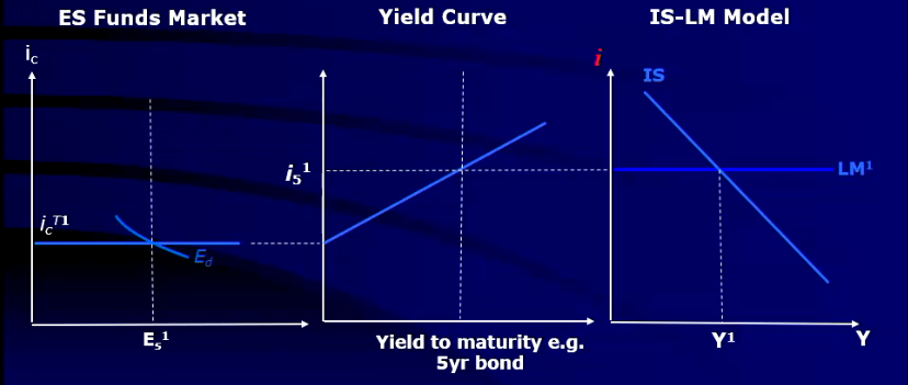
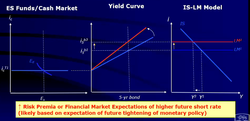
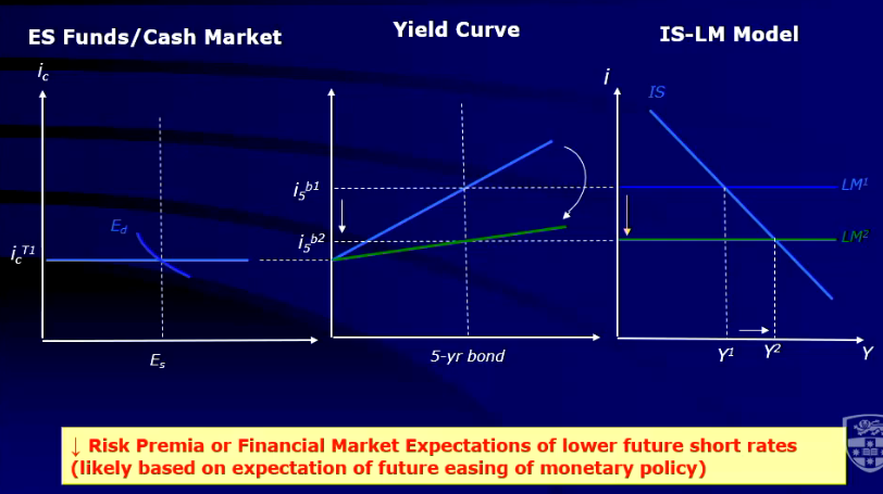
Page 16 - what can risk premia does to yield curve and IS_LM

• Financial Market Changes:

  • Changes in risk premia affect the yield curve and IS-LM model dynamics

    

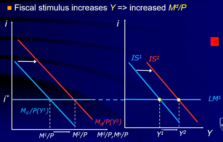
Page 17 - Fiscal policy impacts on IS-LM curve

• Fiscal Policy Impacts:

  • Changes in government spending and taxation affect the IS curve

  • Fiscal stimulus increases output and money demand

    

Page 18 - monetary policy accommodation

• Monetary Policy Accommodation:

  • Increased demand for money met by an increase in money supply at fixed interest rates.

  • Potential upward pressure on prices as the economy approaches full employment

Page 19 - crowding out effect

• Crowding-Out Effects:

  • Zero crowding-out occurs when the economy is below full employment

  • Crowding-out only occurs when income exceeds full employment output

Crowding Out refers to a situation in economics where increased government spending leads to a reduction in private sector spending. This occurs because government borrowing raises interest rates, making it more expensive for businesses and consumers to borrow. As a result, private investment may decline, offsetting the intended stimulative effects of government spending.

Page 24 - two-speed economy definition

• Two-Speed Economy:

  • Higher interest rates and strong currency affecting non-resource sectors

Page 25 - summary of IS-LM model

• Key Points of the IS-LM Model:

  • Movements along the IS schedule reflect changes in interest-sensitive aggregate demand

  • Fiscal policy does not systematically impact interest rates

  • Changes in monetary policy shift the LM schedule and affect