Lecture 10

IV Estimation in Simple Regression

• Regression Model:
  yt = \alpha + \beta xt + u_t

  • Assumption: {Cov}(xt, ut) ≠ 0

  • Existence of Instrument: Variable z_t such that:

  • {Cov}(xt, zt) ≠ 0 (Relevance)

  • {Cov}(zt, ut) = 0 (Validity)

• IV Estimators:
  

  

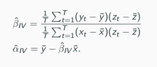
Properties of the IV Estimator

• Consistent Estimators (TS1 - TS3):

  • \hat{\alpha}_{IV} is a consistent estimator of \alpha

  • \hat{\beta}_{IV} is a consistent estimator of \beta

• Statistical Inference Result:
  \sqrt{T}(\hat{\beta}{IV} - \beta) \sim N(0, Var((zt - E(zt))ut)/Cov(xt, zt)^2) \text{ approximately}

• Conditional Variance:

  • If Var(ut|zt) = E(ut^2|zt) = \sigma^2 (Homoskedasticity),

  • Var((zt - E(zt))ut) = \sigma^2 Var(zt)

    • In this case,
      \sqrt{T}(\hat{\beta}{IV} - \beta) \xrightarrow{d} N(0, \frac{\sigma^2 Var(zt)}{Cov(xt, zt)^2})

Other Issues Related to Stochastic Regressors

• Model Specification:

  • Regression Model:
    yt = \alpha + \beta xt + u_t

• Assumptions Violations:

  1. E[ut|xt] = 0

  2. Var(ut|xt) = \sigma^2

  3. (xt, ut) is iid

• If E[ut|xt] \neq 0 (Exogeneity Violation):

  • OLS Estimator fails.

Conditional Heteroskedasticity

• If Var(ut|xt) = \sigma^2t \neq \sigma^2 , the variance depends on xt .

• Implications for OLS Estimator:

  • Unbiased:
    \hat{\beta} = \frac{\sum{t=1}^T (xt - \bar{x})(yt - \bar{y})}{\sum{t=1}^T (x_t - \bar{x})^2}

  • Error:
    \hat{\beta} - \beta = \frac{\sum{t=1}^T (xt - \bar{x})(ut - \bar{u})}{\sum{t=1}^T (x_t - \bar{x})^2}

  • Therefore, E[\hat{\beta} - \beta|x_t] = 0

• Variance of the OLS Estimator:

  • When no conditional heteroskedasticity:
    Var(\hat{\beta}|xt) = \sigma^2 \frac{1}{\sum{t=1}^T (x_t - \bar{x})^2}

  • Estimated by s^2 instead of \sigma^2

Statistical Inference under Heteroskedasticity

• Use of Robust Standard Errors:

  • Remedies for heteroskedasticity: use White’s or HAC Standard Errors.

  • Hypothesis Testing and Confidence Intervals are then valid.

Conditional Autocorrelation

• Definition:

• Correlation of Errors:
  Cor(ut, us) = \frac{Cov(ut, us)}{\sqrt{Var(ut)Var(us)}}

• Implies OLS Estimator is unbiased but requires a careful derivation for the standard error.

Basics on Time Series

• Importance in Economics:

• Key Models: - Autocorrelation in linear regression framework must be understood.

Autocovariance and Autocorrelation

• Definitions:

  • Autocovariance:
    \gamma{t,s} = E[(Xt - \mu)(X_s - \mu)]

  • Autocorrelation:
    \rho{t,s} = \frac{\gamma{t,s}}{\sigma^2}

Stationary Time Series

• Definitions of Stationarity:

  • Strictly Stationary: Joint distributions invariant under time shifts.

  • Weakly Stationary: Mean, Variance constant, Autocovariance depends only on lag.

• Autocovariance Function:
  \gamma(h) = E((Xh - \mu)(X0 - \mu))

Examples of Time Series Models

• White Noise:
  E(Xt) = 0 and Var(Xt) = \sigma^2

• Moving Average Processes (MA(1)):
  Xt = \epsilont - \theta \epsilon_{t-1}

AR(p) Models

• Model Specification:
  Xt = \mu + \phi1 X{t-1} + \ldots + \phip X{t-p} + \epsilont

AR(1) Model and Covariance Stationary

• Condition for Stationarity: |\phi1| < 1 \Rightarrow Cov(Xt) \text{ stationary}

  • If |\phi_1| \geq 1 , series is generally not stationary, exemplified by random walk behaviour.