DSCI NOTES Week 1-6
Week 1: Introduction to Data Analysis
Types of Data Analysis Questions
Descriptive: Summarizes characteristics of a data set without interpretation.
Example: "How many people live in each province and territory in Canada?"
Exploratory: Looks for patterns, trends, or relationships in a single data set.
Example: "Does political party voting patterns change with indicators of wealth in a set of data collected on 2,000 people living in Canada?"
Predictive: Focuses on predicting outcomes based on existing data.
Example: "What political party will someone vote for in the next Canadian election?"
Inferential: Examines if findings from a single data set can apply to the wider population.
Example: "Does political party voting change with indicators of wealth for all people living in Canada?"
Analysis Tools
Summarization: Computes and reports aggregated values.
Example Question: "What is the average race time for runners in this data set?"
Visualization: Graphically plots data for interpretation.
Example Question: "Is there any relationship between race time and age for runners in this data set?"
Classification: Predicts a class/category for new observations.
Example Question: "Given measurements of a tumor's average cell area and perimeter, is the tumor benign or malignant?"
Regression: Predicts a quantitative value for new observations.
Example Question: "What will be the race time for a 20-year-old runner who weighs 50kg?"
Clustering: Finds unknown/unlabelled subgroups in a dataset.
Example Question: "What products are commonly bought together on Amazon?"
Estimation: Taking measurements or averages from a smaller group to a larger population.
Example Question: "Given a survey of cellphone ownership of 100 Canadians, what proportion of the entire Canadian population own Android phones?"
Data Science: use of reproducible + auditable processes to get value from data
Reproducible: easily repeated by others
Auditable: easily traced & critiqued
Data Set Structure
Data Set: Structured collection of numbers and characters.
Rows: Represent observations (horizontal).
Columns: Represent variables (vertical).
Data Frame: is specifically a data set with the row type
R Messages and Functions
Loading the
tidyversein R can produce messages about attached packages and potential conflicts.Users can access specific versions of functions from loaded packages by using the package prefix (e.g.,
dplyr::filter()).
Naming Conventions in R
Use lowercase letters, numbers, and underscore (_).
Avoid using spaces or special characters.
R is case-sensitive.
Use meaningful variable names for better readability of scripts.
Filtering and Selecting Data: Filter THEN Select
The
filter()function: obtain subset of ROWS with specific valuesExample:
filter(data_frame, logical statement)will return a new data frame with logical statement evaluated to TRUE .
The
select()function extracts specific COLUMNS from the data frame.
Mutating Data
The
mutate()function adds/modifies columns in a data frame, allowing for new calculations or transformations of existing data.
Data Visualization with ggplot
ggplot()is a function used for creating visualizations in R, with layering concepts similar to how one builds a plot manually.
Week 2: Reading Data
Advantages of using R:
statistical analysis functions go beyond Excel
free & open-source
transparent & reproducible code
can handle large amounts of data + complex analyses
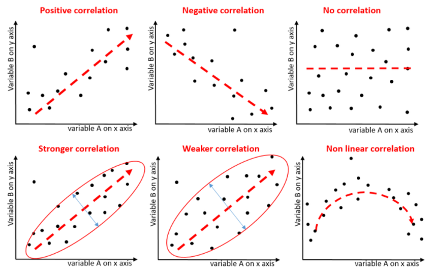
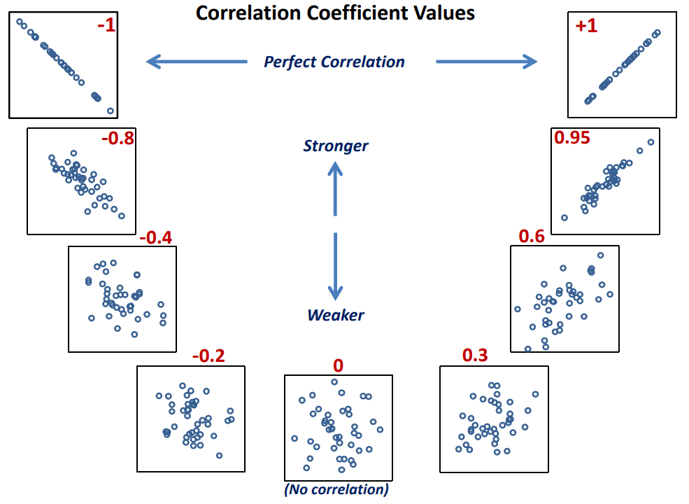
Correlation does not equal causation: Even if a correlation existed, it wouldn't necessarily mean that one variable causes the other. There could be other factors influencing both variables.
More data and analysis: To make a more definitive conclusion, it would be helpful to have more data points and conduct statistical tests to quantify the strength and significance of any potential correlation
Types of File Paths
Path: where the file lives on computer, the directions to the file
Local (computer):
Absolute path: locates file with respect to the “root” folder on computer
full path from the root folder to the file's location on the filesystem
STARTS with /
e.g. /home/instructor/documents/timesheet.xlsx
Relative path: locates a file relative to your working directory
DOESN’T start with /
e.g. documents/timesheet.xlsx
Working directory: current folder/location containing the file we are currently working on, serving as reference point for relative paths
Format DOESN’T include the working directory
Use to navigate files efficiently & ensures code can be run on diff computer
Remote (on web):
Uniform Resource Locator (URL):A specific type of address used to access resources on the internet, which includes the protocol, domain name, and path to the resource.
http:// or https://
assign it to object named url to use it:
url <- "https://raw.githubusercontent.com/UBC_DCSI/data/main/can_lang.csv"
canlang_data <- read_csv("url")
canlang_data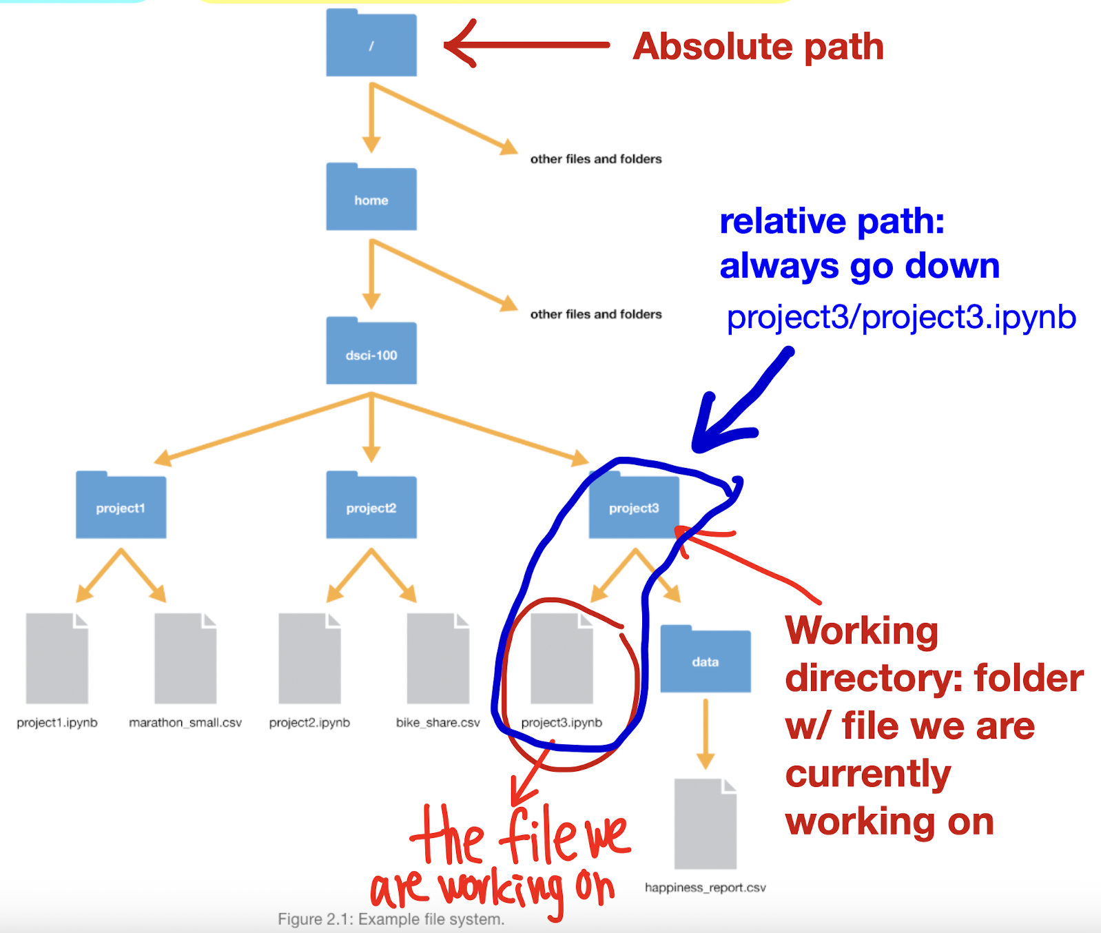
Ex. if absolute path looks like: /Users/my_user/Desktop/UBC/BIOL363/SciaticNerveLab/sn_trial_1.xlsx
and working directory is UBC, relative path: BIOL363/SciaticNerveLab/sn_trial_1.xlsx
Loading data from computer (Workflow): DO IT CAREFULLY
Navigate file, see what it looks like: column names? delimiters? lines to skip?
Prepare to load into R
skim data, might need to modify, look at how values are separated
might need to load a
library, download file, or connect to database
Load into R: check with reading data function
Inspect the result CAREFULLY to make sure it worked: to reduce bugs + speed up
Reading Data Functions
read_csv(): To read CSV files (commas as the delimiter)read_tsv(): To read tab-separated files (tabs between the columns)read_delim(): For flexibility in choosing different delimiters, can import both CSV and TSV files, but just SPECIFY WHICH DELIMITER during import1. specify path to file as first argument
2. provide tab character
“\t"as delim argument3. set col_names argument to FALSE to say there’s NO COLUMN NAMES GIVEN in data, if
TRUEfirst row will be treated as column namese.g.
canlang_data <- read_delim("data/can_lang_no_names.tsv", delim = "\t", col_names = FALSE)
read_excel(): For reading Excel spreadsheets, loadreadxlpackage firstsheetargument to specify sheet # or name (when file has multiple sheets)rangeargument to specify cell ranges
Skipping Rows
skip: to ignore non-crucial information at the top of the data files when loading, so data can be read properly
1. Look at data first to see HOW MANY LINES WE DON’T NEED (e.g. if columns start at line 4, skip the first 3 lines)
canlang_data <- read_csv("data/can_lang_meta-data.csv", skip = 3)
Working with Databases (SQLite, PostgreSQL)
Connect to databases using
dbConnect()and run SQL queries through R without needing extensive SQL knowledge, thanks to packages likedbplyr.
Use
collect()to bring data from a database into R as a data frame for local analysis.
We DIDN’T get a data frame from the database, but it’s a REFERENCE (data still stored in SQLite database)
Reading data from database
In order to open a database in R, you need to take the following steps:
Connect to the database using the
dbConnectfunction.library(DBI) #when using SQLite Database canlang_conn <- dbConnect(RSQLite::SQLite(), "data/can_lang.db")library(RPostgres) #when using PostgreSQL Database canmov_conn <- dbConnect(RPostgres::Postgres(), dbname = "can_mov_db", host = "fakeserver.stat.ubc.ca", port = 5432, user = "user0001", password = "abc123")For PostgreSQL, there’s additional info needed to include:
host: URL pointing to where database is locatedport: communication endpoint btwn R and PostgreSQL databaseCheck what tables (similar to R dataframes, Excel spreadsheets) are in the database using the
dbListTablesfunctionOnce you've picked a table, create an R object for it using the
tblfunctionMake sure you
filter&selectdatabase table before usingcollect
Writing Data to Files
Use
write_csv()to save processed data frames back to CSV format after analysis.
strings in R: Strings in R are sequences of characters used to represent text data. They can be created using single or double quotes.
Function | Description |
| To read CSV files. |
| To read CSV files, but uses ; for field separators and , for decimal pts |
| To read tab-separated files. |
| For flexibility in choosing different delimiters. |
| For reading Excel spreadsheets. |
| To save processed data frames back to CSV format.
|
| Connect to databases. |
| Bring data selected from a database into R as a data frame.
|
| To obtain a subset of ROWS w/ specific values
if there’s multiple CONDITIONS, you can JOIN THEM USING COMMA or & ex. |
| Extract specific COLUMNS from the data frame.
can also do |
| Adds or modifies columns in a data frame.
expression example: |
| Function used for creating visualizations in R. |
| Adds specified title to the plot |
| To load package into R, to use its functions and datasets available |
| For comments, R will ignore any text after the symbol |
| To rename columns, use subsequent argument |
| Use when data at URL is not formatted nicely, then can use read_ 1st argument: url, 2nd: path we want to store downloaded file |
| To list all names of tables in database
|
| To reference a table in the database (allows us to perform operations like selecting columns etc.) ex. |
| To count how many times a specific value appears in a column
|
| Argument to specify sheet # or name Argument to specify cell ranges
|
| Used to specify the location of a file on computer or on web when reading data into R, format of path varies depending on if it's local or remote file: when URL, assign it first:
|
| Replaces spaces w/ underscores & convert to lowercase to make it standard format
|
| Order rows by the values of the given columns (default is increasing)
|
| Used to modify the non-data components of the plot with specified options
|
| SELECTS ROWS according to their row number, keep rows in the given range ex. we want rows 1 to 10 |
| Keep the n rows with the LARGEST values of a variable
|
| Keep the n rows with the SMALLEST values of a variable
|
| To preview the first 6 rows of dataframe |
| To preview last 6 rows of dataframe |
| Counts the number of rows in a table’s group e.g. column has names of restaurants and we want to find the count for each restaurant name |
| Organizes a variable based on values of second variable e.g. |
| To pull up documentation for most functions |
Week 3: Wrangling
Real-World Data Issues:
Data is often messy:
Inconsistent formats (e.g., commas, tabs, semicolons).
Missing data and extra empty lines.
Split into multiple files (e.g., yearly data).
Corrupted files and custom formats.
Even after loading data in R, it may remain messy.
Key Point: Make data "tidy"
What is Tidy Data?
Tidy data enhances: Reproducibility, Efficiency, Collaboration
Tidy datasets are organized with multiple variables; messy datasets are typically structured in a single column.
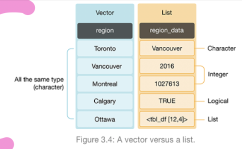
Data Structures in R:
Vectors: An objects that contains collections of ordered elements of the SAME DATA TYPE
Create using the
c()function
Lists: Ordered collections that can contain MIXED TYPES of elements.
Data Frame as a Special List:
Characteristics of Tidy Data
Variables should be in columns
Each row should represent a single observation
Each cell is single measurement
Easier manipulation, plotting, and analysis in consistent formats.
Examples of Tuberculosis Data
Different representations of tuberculosis data are analyzed for tidiness.
Analysis Results:
Example structures of data:
Tidy Data:
Country,Year,Cases,PopulationComplies with tidy data principles (each variable in its own column).
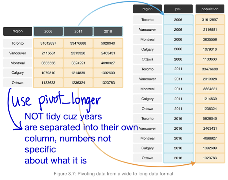
Not Tidy Data:
Columns with non-specific names or multiple values in one column (e.g., year grouped with cases and population).
Requires restructuring to be considered tidy
Tools for Tidying and Wrangling Data
Focus on
tidyversepackage functions:dplyr functions:
select,filter,mutate,group_by,summarize
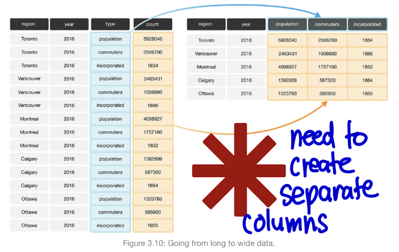
tidyr functions:
pivot_longer,pivot_wider
purrr function:
map_dfr
Step-by-Step Data Transformation
Examples using library functions demonstrated with
penguinsdataset.Key functions:
Select: Choose columns from a data frame.
Filter: Subset rows based on conditions (e.g., flipper length).
Mutate: Transform existing columns or create new columns (e.g., mass conversion).
Chaining Operations with R
Discussed methods to handle multiple operations:
Saving Intermediate Objects:
Drawbacks include complexity and potential memory issues.
Composing Functions:
Disadvantage: Less readable due to inner function execution first.
Using Pipes (
|>):Enhances readability and avoids intermediate variables.
Grouping and Summarizing Data: group_by() + summarize()
Concepts:
Grouping data based on COLUMN VALUES.
Summarizing is when you COMBINE DATA into fewer summary values (e.g., average pollution).
Applications to
penguinsdataset: average mass by species.
Introduction to Iteration
Iteration Defined:
Executing a process multiple times (e.g., in data manipulation).
map_dfrFunctionality:Example of iterating over multiple columns in the
penguinsdataset.Caution on the multiplicity of
map_variants available.
Other
na.rm in R: Argument in functions to handle missing values (NA).
Purpose: Specify whether to remove NA values before computation.
Usage: Set to
TRUEto ignore NAs, allowing calculations on available data.Example:
mean(x, na.rm = TRUE)calculates the mean while excluding NAs.Importance: Useful for accurate analysis in datasets with missing values.
Operators for Data Wrangling:
Comparison:
==: Extracting rows w/ certain value, checks for equality btwn two values, returning true if equal and false otherwise!=: Extracting rows that DON’T have certain value, means NOT EQUAL TO<: Look for values BELOW a threshold<=: Look for values EQUAL TO OR BELOW a threshold>: Look for values ABOVE a threshold>=: Look for values EQUAL TO OR ABOVE a threshold
Logical:
%in%: Extracting rows w/ values in vector, used to see if an value belongs to a vector!: Means NOT, changing TRUE to FALSE and FALSE to TRUE&: Extracting rows satisfying multiple conditions, works just like the comma|: Vertical pipe to give cases where one condition or another or both are satisfiede.g.
filter(official_langs, region == "Calgary" | region == "Edmonton")
%>%: sends result of one function to the next function
Functions for Data Wrangling
Function | Description |
| Transform data FROM WIDE TO LONG FORMAT
|
| Convert data FROM LONG TO WIDE FORMAT
|
| Split a single column into multiple columns by delimiter.
|
| Generate summary statistics on columns
|
dfr is for data frames, combining row-wise | Apply functions to each element in list/vector & returns results as single data frame
DOESN’T have an argument to specify which column to apply functions to, so use select beforehand |
| To group by one or more variables
|
| Apply functions to MULTIPLE COLUMNS simultaneously e.g. |
| Applies functions across COLUMNS WITHIN ONE ROW |
concatenate | To CREATE VECTORS/COLUMNS
|
| Filtering data frames based on matches in another data frame |
| To convert data in numeric format |
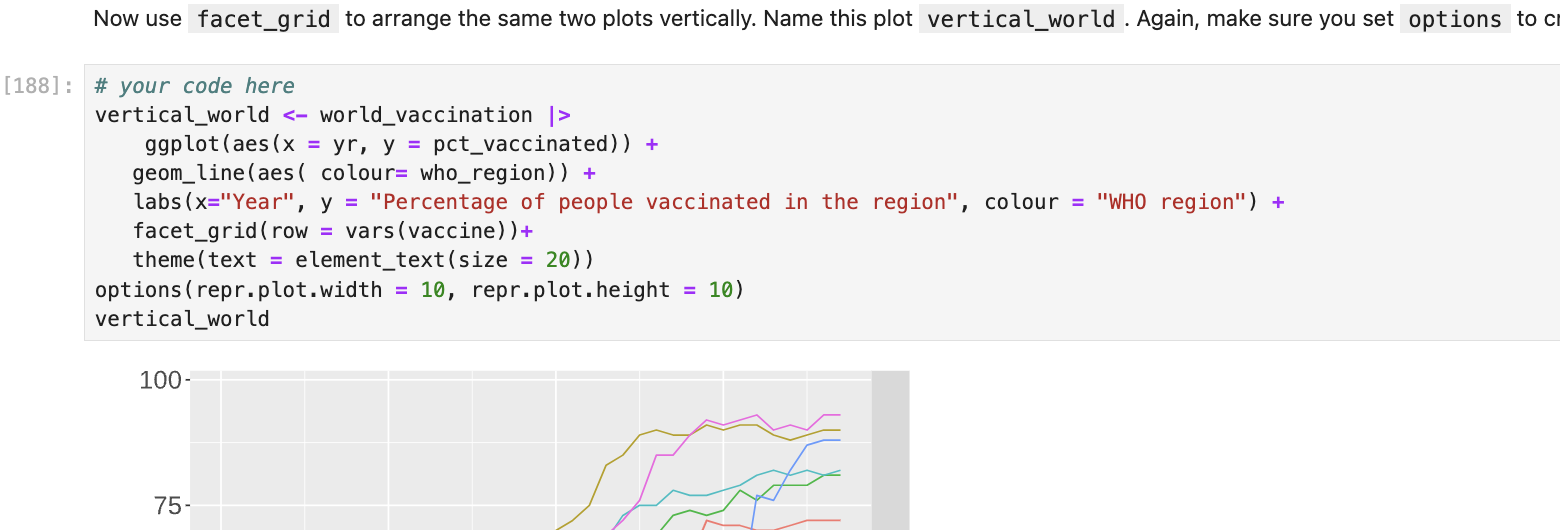
| To have plots side by side for comparison
|
Week 4: Visualization
Designing Visualizations
Questions driving visualization: Each visualization should aim to answer a specific question from the dataset.
Clarity and Greatness: A good visualization answers a question clearly, while a great one hints at the question itself.
Types of questions answered through visualizations:
Descriptive: E.g., What are the largest 7 landmasses on Earth?
Exploratory: E.g., Is there a relationship between penguin body mass and bill length?
Other types: inferential, predictive, causal, mechanistic.
Creating Visualizations in R
ggplot2: Key components include:
Aesthetic Mappings (
aes): map dataframe columns to visual propertiesGeometric Objects (
geom): encode HOW TO DISPLAY those visual propertiesScales: transform variables, set limits
Elements are combined using the
+operator.
Types of Variables
Categorical Variables: can be divided into groups (categories) e.g. marital status
Quantitative Variables: measured on numeric scale (e.g. height)
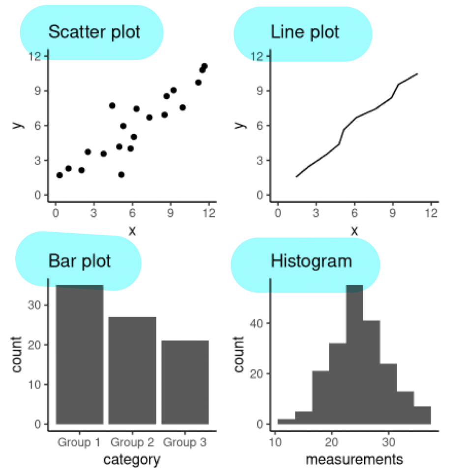
Visualization Types
Scatter Plots
To visualize relationship between 2 QUANTITATIVE variables
Example Question: How does horsepower affect the fuel economy of an engine?
Line Plots
To visualize TRENDS w/ respect to an INDEPENDENT QUANTITY (e.g. time)
Example: Changes in atmospheric CO2 levels over the last 40 years.
Bar Plots (there’s SPACING BETWEEN BARS)
To visualize COMPARISON of AMOUNTS
Example: Number of students in each faculty (sci, bus, med, arts)
Histograms (NO space between bars)
To visualize DISTRIBUTION OF SINGLE QUANTITATIVE VARIABLE
Example: Differences in life expectancy across continents in 2016.
Rules of Thumb for Effective Visualizations
Avoid using tables, pie charts, and 3D visualizations for clarity and simplicity
Use color palettes that are simple and colorblind-friendly
A great visualization conveys its story without requiring additional explanation
Refining Visualizations
Convey message, minimize noise
use legends and labels
ensure text is big enough to read and clearly visible
be wary of overplotting
Explaining the Visualization
Presented visualizations should form a narrative:
Establish the setting and scope.
Pose the question.
Use the visualization to answer the question.
Summarize findings and motivate further discussion.
Saving the Visualization
Choose appropriate output formats based on needs:
Raster Formats: 2D grid, often compressed before storing so takes less space
JPEG (
.jpg, .jpeg): lossy, usually for photosPNG (
.png): lossless, usually for PLOTS / LINE drawingsBMP (
.bmp): LOSSLESS, RAW IMAGE data, no compression (rarely used)TIFF (
.tif, .tiff): typically lossless, no compression, used mostly in graphic arts, publishing
Vector Formats: collection of mathematical objects (lines, surfaces, shapes, curves)
SVG (
.svg): general purpose useEPS (
.eps): general purpose use, infinitely scaleable great for presentation
Function | Description |
| To make scatterplot |
| To make line plot |
| To make histogram |
| To make bar graph |
| Adds VERTICAL line to a plot, to INDICATE SPECIFIC X-AXIS e.g. threshold, average |
| Adds HORIZONTAL line to a plot, to INDICATE SPECIFIC Y-AXIS e.g. threshold, average |
| To create aesthetic mapping |
| To create geometric object |
| Sets limits for x-axis/y-axis in plot, controls range of values displayed |
For aes mapping, fills in BARS by specific color or separates counts by a variable aside form the x/y axis | |
| Prevents chart from being stacked, PRESERVES VERTICAL position of plot while adjusting horizontal position |
| To distinguish different groups/categories by color |
| Allows further visualization by varying data points by shape |
| For labels, axes |
| To create a plot that has MULTIPLE SUBPLOTS arranged in grid e.g.
|
| To save plots in various formats |
| To create line break in axis names |
| For fill aes w/ CATEGORICAL variable |
| For fill aes w/ NUMERIC variable |
| To accomplish logarithmic scaling when AXES have LARGE number, also FORMAT AXIS LABELS to increase readability e.g. |
| name of the column we want to use for comparing e.g. |
| In aes mapping, to reorder factors based on values of another variable e.g. |
| Convert variables to factor type Factor: data type used to represent categories |
Other
add
alpha = 0.2togeom_pointto enhance visibility when points overlaptheme(text = element_text(size = 12), legend.position = "top", legend.direction = "vertical")options(repr.plot.width = 8, repr.plot.height = 8)to set plot sizegeom_bar(stat = "identity")to DISPLAY VALUES in data frame AS ISgeom_bar(position = "identity")to DISPLAY BARS exactly as they are w/o any stacking or dodginggeom_vline(xintercept = 792.458, linetype = "dashed")to make certain lines stand outgeom_histogram(bins, binwidth)
Week 5: Version Control
What’s Version Control?
Version Control: the process of keeping a record of changes to documents, indicating changes made, and who made them
View earlier versions and revert changes
Facilitates resolving conflicts in edits.
Originally for software development, but now used for many tasks
Why Do We Need Collaboration Tools?
Initial approach: Sending files to teammates via email.
Problems:
Unclear versioning and edit tracking.
No insight into who made edits or when.
Difficulty in reverting to prior versions.
Poor communication regarding tasks and issues.
Alternative approach: Sharing via Dropbox/Google Drive.
Limitations:
Simple version management but lacks:
Edit tracking (who, when).
Clarity on project status after extended periods.
Easy means to revert changes.
Organized discussions for tasks/issues.
Complicated file naming like "final_revision_v3_Oct2020.docx" instead of clear version history.
Git and GitHub
Git → Version Control Tool
Tracks files in a repository (folder that you tell Git to pay attention to)
Responsible for keeping track of changes, sharing files, and conflict resolution
Runs on local machines of all users
GitHub → Cloud Service, Online Repositories
Cloud service that hosts repositories
Manages permissions (view/edit access)
Provides tools for project-specific communication (issues tracking)
Can build and host websites/blogs
Version Control Repositories
Two copies of the repository are typically created:
Local Repository: Personal working copy on OWN COMPUTER
Remote Repository: Copy of project hosted on server ONLINE, for sharing w/ others
Both copies maintain a full project history with commits (snapshots of project files at specific times).
Commits include a message and a unique hash as identifiers.
Key Concepts and Commands
Overview of important files and areas:
Working Directory: Files like
analysis.ipynb,notes.txt, andREADME.mdon the local computer.Staging Area: Where changes are prepared for a commit (
.git).Remote Repository: GitHub stores your files.
Version Control Workflows
Committing changes: Save your changes in the local repo
Working Directory: Contains files that may have pending changes
Git Add: command to stage selected files to prepare for committing
Typical files to stage:
analysis.ipynb,README.md.
Git Commit: takes snapshot of files in the staging area, recording changes
Includes message to describe the nature of the changes
Pushing changes: Share commits with remote repo
Git Push: UPLOAD UPDATES to the REMOTE repo on GitHub
Keeps COLLABORATORS SYNCHRONIZED w/ latest changes
When want to back up work
Pulling changes: COLLECTING NEW CHANGES others added on remote repo to your local machine
Git Pull: download file to computer
To SYNCHRONIZE LOCAL repo w/ changes made by collaborators on the remote repo
Cloning a repo: copy/download ENTIRE CONTENT (files, project, history, location of repo) of a REMOTE server repo to LOCAL MACHINE
Git Clone: creates connection between local and remote repo
To GET a WORKING COPY of repo
Other
Git has distinct step of adding files to staging area:
Not all changes made are ones we want to push to remote GitHub repo
Allows us to edit multiple files at once
Associate particular commit message w/ particular files (so they specifically reflect changes made)
GitHub Issues: NOT ideal for specific project communication
Issues only persist while they are open, deleted when closed
CAN CLONE/PULL from any PUBLIC remote repo on GitHub, BUT can only push to public remote repo YOU OWN or have ACCESS to
Editing files on GitHub w/ pen tool: reserved for small edits to plain text files
Generate GitHub personal access token to authenticate when sending/retrieving work
Good practice to pull changes at start of every work session before working on local copy
Handling merge conflicts: open offending file in plain text editor & identify conflict markers (
<<<<<<<, =======, >>>>>>>)Manually edit file to resolve the conflicts, ensuring to keep the necessary changes from both versions before saving & committing resolved file
Week 6: Classification 1 - Using K-Nearest Neighbours
Classification Concept
Example: Diagnosing cancer tumor cells
Labels: "benign" or "malignant"
Questions arise about new cases based on features (e.g., Concavity and Perimeter)
Classification methods aim to answer questions regarding labels based on data
K-Nearest Neighbours (KNN) Classification
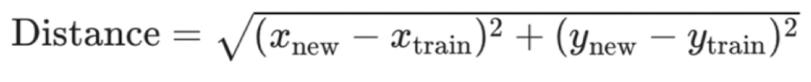
Predict label/class for a new observation using K closest points from dataset
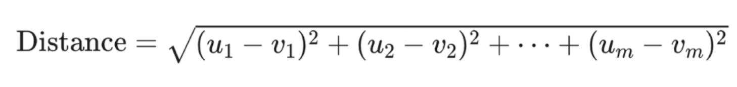
Compute distance between new observation and each observation in training set, to find K nearest neighbours
can go beyond 2 predictors
Sort data in ascending order according to distances
Choose the top K rows as “neighbors”
Classifying new observation based on majority vote
Tidymodels Package in R
tidymodels: Collection of packages and handles computing distances, standardization, balancing, and prediction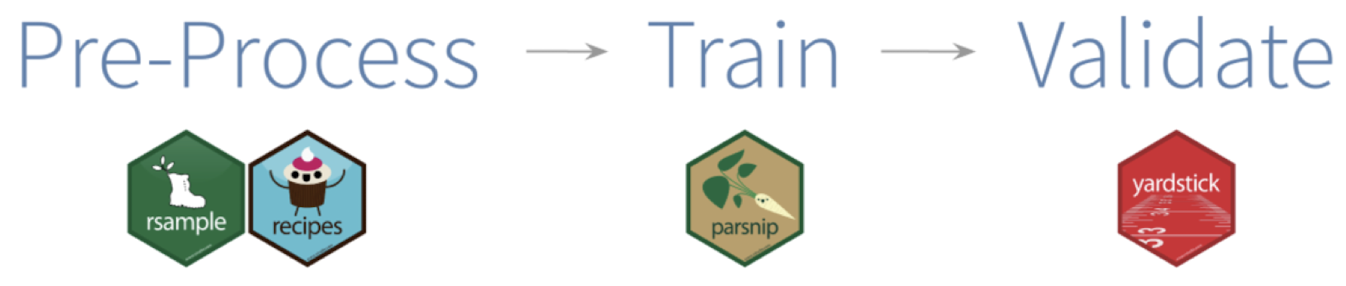
Load the libraries and data
Necessary libraries include
tidyverseandtidymodelsImport data and mutate as necessary
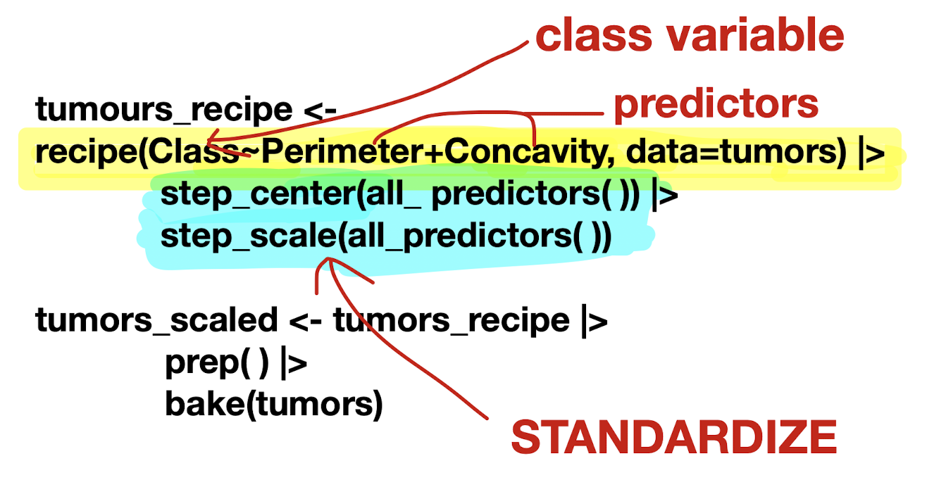
Make a
recipeto specify predictors/response and preprocess data
recipe(): Main argument in formulaArguments: formula and data
prep()&bake()
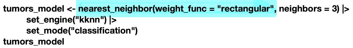
Build model specification (
model_spec) to specify model and training algorithmmodel type: kind of model you want to fit
arguments: model parameter values
engine: underlying package the model should come from
mode: type of prediction
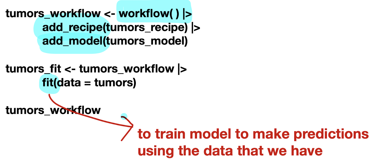
Put them together in a workflow and then fit it
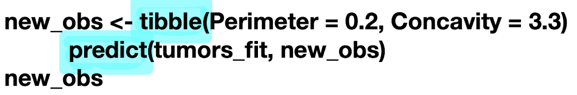
Predict a new class label using
predict
Importance of Standardization
Standardization: important to account for all features in distance calculation, enhances prediction accuracy
Adjusting for center and spread
Shift and scale data to carry average of 0 and standard deviation of 1
Non standardized Data:
Issues arise if one variable's scale is significantly larger than others
Function | Description |
| To prepare data for modelling task |
| Centers numeric variables and standardize data |
| Scales numeric variables and standardize data |
| Prepares recipe for modelling by estimating required values from training data |
| Applies preprocessing steps to new data |