Chapter 3: Descriptive Statistics

3.1 Samples and Populations

Sample: refers to a selection of individual people or items from a population

Population: consists of all possible people or items who/which have a particular characteristic

• Researchers are only interested in what the samples can tell them about the populations, therefore, it is important that we ensure the any samples used in the research are truly representative of the target population.

Experimenter Bias: the experimenters subconsciously chose to follow people who help support their hypothesis

Parameters: descriptions of populations

Statistics: descriptions of samples

• We often use sample statistics as estimations of population parameters.

3.2 Measures of Central Tendency

Measures of Central Tendency: give us an indication of the typical score in our sample; effectively an estimate of the middle point of our distribution of scores

3.2.1 Mean

Mean: the sum of all the scores in a sample divided by the number of scores in that sample

Example:

mean of the sample of the 4 scores: 5, 6, 9, 2

(5 + 6 + 9 + 2) / 4 = 5.5

3.2.2 Median

Ranking: where we arrange a set of scores in ascending order and then assign a position number (rank) to each one

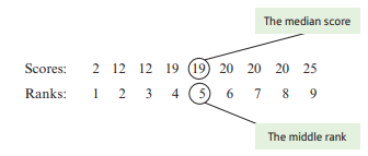
Median: the middle score/value once all scores in the sample have been put in rank order

Example 1:

median for the sample: 2, 20, 20, 12, 12, 19, 19, 25, 20

Example 2:

median for the sample: 2, 12, 12, 19, 19, 20, 20, 20, 25, 26

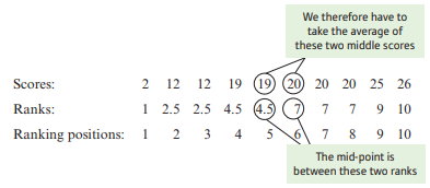
• If there are even number of scores, the median will be between the 2 middle scores. Therefore, the median in this example will be the average of the 2 scores in the 5th and 6th positions: (19 + 20) / 2 = 19.5

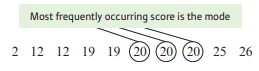
3.2.3 Mode

Mode: the most frequently occurring score in a sample

3.2.4 Which measure of central tendency should you use?

• The important point to keep in mind when choosing a measure of central tendency is that it should give you a good indication of the typical score in your sample.
• The mean is the most frequently used measure of central tendency and it is the one you should use once you are satisfied that it gives a good indication of the typical score in your sample. It is the measure of choice because it is calculated from the actual scores themselves, not from the ranks, as is the case with the median, and not from frequency of occurrence, as is the case with the mode.
  • Problem with the Mean: because the mean uses all the actual scores in its calculation, it is sensitive to extreme scores.
• If you find that you have extreme scores and you are unable to use the mean, then you should use the median. The median is not sensitive to extreme scores because it is simply the score that is in the middle of the other scores when they are put in ascending order.
• As the mode is simply the most frequently occurring score, it does not involve any calculation or ordering of the data.

3.2.5 The Population Mean

• One way of estimating the population mean is to calculate the means for a number of samples and then calculate the mean of these sample means.

3.3 Sampling Error

Sampling Error: the difference between the population parameter and the sample statistic; the degree to which sample statistics differ from the equivalent population parameter

• Whenever we select a sample from a population, there will be some degree of uncertainty about how representative the sample actually is of the population. Thus, if we calculate a sample statistic, we can never be certain of the comparability of it to the equivalent population parameter.

3.4 Graphically Describing Data

Exploratory Data Analysis (EDA): where we explore the data that we have collected in order to describe it in more detail. These techniques simply describe our data and do not try to draw conclusions about any underlying populations.

3.4.1 Frequency Histogram

Frequency Histogram: a graphical means of representing the frequency of occurrence of each score on a variable in our sample. The x-axis contains details of each score on our variable and the y-axis represents the frequency of occurrence of those scores.

• The frequency histogram is a good way for us to inspect our data visually.

  

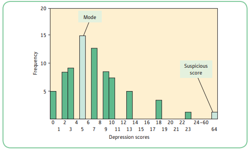
• The frequency histogram is useful for discovering other important characteristics of your data. In addition, your histogram gives you some useful information about how the scores are spread out; that is, how they are distributed.

• The best way of generating a histogram by hand is to rank the data first. You then simply count up the number of times each score occurs in the data; this is the frequency of occurrence of each score.

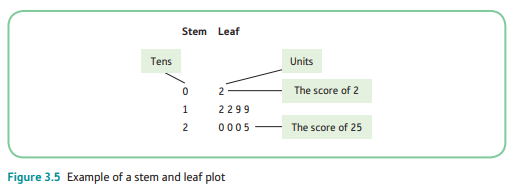
3.4.2 Stem and Leaf Plots

Stem and Leaf Plots: similar to histograms but the frequency of occurrence of a particular score is represented by repeatedly writing the particular score itself rather than drawing a bar on a chart

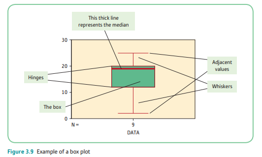
3.4.3 Box Plots

Box Plots/Box and Whisker Plots: enable us to easily identify extreme scores as well as seeing how the scores in a sample are distributed.

Outliers/Extreme Scores: those scores in our sample that are a considerable distance either higher or lower than the majority of the other scores in the sample

• One of the limitations of box plots is that it is often more difficult to tell when a distribution deviates from normality.

  • Guide:
  • Normally distributed data: equal whiskers coming from both edges of the box
  • Negatively skewed data: no whisker coming from the top of the box

  

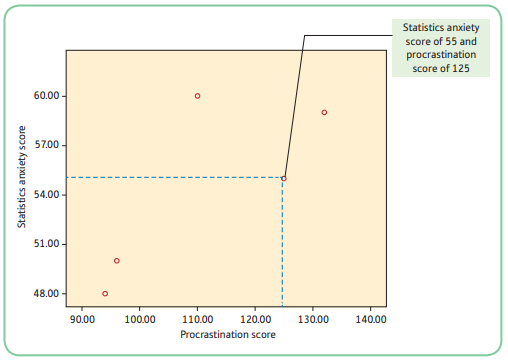
3.5 Scattergrams

Scattergram: gives a graphical representation of the relationship between 2 variables. The scores on one variable are plotted on the *x-*axis and the scores on another variable are plotted on the y-axis.

3.6 Sampling Error and Relationships between Variables

• The conclusions we draw from sample data are subject to sampling error. We can rarely be certain that what is happening in the sample reflects what happens in the population.
• The larger the sample we take from the population, the more likely it is that it will reflect that population accurately.

3.7 The Normal Distribution

Normal Distribution: a distribution of scores that is peaked in the middle and tails off symmetrically on either side of the peak; the distribution is often said the be ‘bell-shaped'; for a perfectly normal distribution, the mean, median and mode will be represented by the peak of the curve.

For a distribution to be classed as normal it should have the following characteristics:

• It should be symmetrical about the mean.

• The tails should meet the x-axis at infinity.

• It should be bell-shaped.

• Once we have the mean and standard deviation, we can plot the normal distribution by putting these values into a formula.

• The more scores from naturally occurring variables you plot, the more like the normal distribution they become.

3.8 Variation or Spread of Distributions

Variance or Variation of Scores: indicates the degree to which the scores on a variable are different from one another.

3.8.1 The Range

Range: the highest score in a sample minus the lowest score

• Although the range tells us about the overall spread of the scores, it does not give us any indication of what is happening between these scores.

3.8.2 Standard Deviation

Mean Deviation: gives us an indication of how much the group as a whole differs from the sample mean; to calculate, we have to sum the individual deviations and divide by the number of scores we have.

• Problem with the Mean Deviation: Approximately half of the deviations from the mean will be negative deviations (the scores will be less than the mean) and half will be positive deviations (the scores will be greater than the mean). If we sum these deviations, we will get 0.

Variance: the average squared deviation of scores in a sample from the mean

• Problem with the Variance: It is based upon the squares of the deviations and thus it is not expressed in the same unites as the actual scores themselves.

Standard Deviation (SD): the degree to which the scores in a dataset deviate around the mean; it is an estimate of the average deviation of the scores from the mean; the square root of the variance

• Problem with Standard Deviation: It tends to be an under estimate of the population standard deviation, therefore, we usually report a slightly modified version of the sample standard deviation when we are trying to generalize from our sample to the underlying population.

3.9 Other Characteristics of Distributions

Kurtosis: a distribution is a measure of how peaked the distribution is

• Platykurtic: a flat distribution
• Leptokurtic: a very peaked distribution
• Mesokurtic: a distribution between the two extremes
• Positive values of kurtosis on the output suggest that the distribution is leptokurtic, whereas negative values suggest that it is platykurtic. A zero value tells you that you have a mesokurtic distribution.

3.10 Non-normal Distributions

3.10.1 Skewed Distributions

Skewed Distributions: those where the peak is shifted away from the center of the distribution and there is an extended tail on one of the sides of the peak

Negatively Skewed Distribution: the peak has been shifted to the right towards the high numbers of the scale and the tail is pointing to the low number (or even pointing to the negative numbers)

Positively Skewed Distribution: the peak shifted left, towards the low numbers, and has the tailed extended towards the high numbers

• If you come across badly skewed distributions, you should be cautious about using the mean as your measure of central tendency, as the scores in the extended tail will be distorting you mean. In such cases, you are advised to use the median or mode, as these will be more representative of the typical score in your sample.

3.10.2 Bimodal Distributions

Bimodal Distribution: one that has two pronounced peaks; it is suggestive of there being two distinct populations underlying the data

• Essentially, bimodal distributions have two modes, although in most cases the two humps of the distribution will not be equal in height.
• If you come across a bimodal distribution you should look closely at your sample, as there may be some factor that is causing your scores to cluster around the two modal positions.