PSYC STATS EXAM 1 NOTES.docx

CHAPTER 1

80% MC (32 MC questions=80%) 2 problem set 20% Short answer

Variable: characteristic that can change or take on different values

• Most research begins with a general question about the relationship between 2 variables for a specific group. (ex: do psychedelics improve symptoms in depressed adults –v1= psychedelics v2 placebo group)

Population: an entire group of individuals that is defined

• “What is the relationship between [v1] and [v2] among [population]”
• Populations can be very large that they all can’t be examined; almost impossible to represent an entire population

Sample: A sample is used to represent a population

• The goal is to use results from a sample to answer questions about a population
• Sample is generalized to come up with conclusions for population (depends on the degree of confidence)
• Best guess about what is true about this population

Distributions to pay attention to: population frequency distribution, sample of sample distribution and distribution of sample means

Inferential Statistics: use a sample data to make general conclusions (inferences about populations. (ex: presidential polling)

• Sample data provide limited info about the population. Because of this, sample statistics are not perfect representatives of population parameters.

Descriptive statistics: Methods for organizing and summarizing data. (The average)

• Tables or graphs are used (T tests from FRI)

Descriptive value for a

• Population = parameter
• Sample = statistic

Sampling error: The discrepancy between a sample statistic and its population parameter

• Defining and measuring sampling error is a large part of inferential statistics. We care about this bc how close the sample stat to the population parameter we find out through the sampling error.

Data: Measurements obtained in research (ex: height, how fast they can run)

• Goal of stats is to help researchers organize and interpret data

Discrete variables: consist of indivisible categories (ex: a dice roll)

Continuous variables: are infinitely divisible into any unit the researcher chooses (ex.time or weight)

• To establish between variables you must measure the variables we’re interested in
• To do that we choose a scale of measurement

Scale of measurement:

• 4 major scales
• The scale we choose determines the types of questions we can answer with our data

4 scales are..

1. A nominal scale is a unordered set of categories identified by name only (nominolsis=pertaining to name only). Ex: You dont know how much they like it, but you know what they like. (10 like cats 6 like dogs) Only determination you can make is whether the 2 individuals are the same or different on that scale. YOU CANT RANK
2. An ordinal scale is an ordered set of categories. Tells you the direction of difference between 2 individuals. (Ex: Race who won 1st 2nd 3rd) . You only know rank
3. An Intevral scale is an ordered set of equal-sized categories. Identfies both direction and magnitude of a difference. (Temperatures: this is hottest this coldest and provide specific temperature values for each.) More specific than ordinal scale. Zero point is located arbitrary . 0 has no meaning; but each interval has meaning (moving in increments)
4. Ratio scale is like an interval scale where a value of zero indicates none of the variable. This is specific because each increment of change means something different (Ex kelvin: the absence of 0. Allows ratio comparisons of measurements. 0 is meaningful in this scale compared to interval scale; you can divide one measurement by the other (mph; 0 miles = no distance) 0 has a meaning = none of the amount you are measuring

1/27/24

Correlational studies: goal is to determine the strength and direction of the relationship between 2 variables (years of education as a continuous variable); assigned groups

• You are not manipulating the variable; you are just looking at things as they exist naturally
• Correlation does NOT = causation

Experiments: examines the relationship between 2 or more variables by changing 1 variable and observing the effects on the other variable. Assignment is involved= experimental

Makeup:

• Independent variable: a condition or event that is manipulated by the experimenter (I Decide)
• Dependent variable: the aspect or behavior thought to be affected by the independent. variable. Always measured not manipulated. (Depends on what I decide)

Ideally: all other variables are controlled to prevent them from influencing the results

Non-experimental studies: Similar to experiments bc they also compare groups of scores. Key difference: They DO NOT use manipulated variables to differentiate the groups (naturally occurring groups) Are you assigning

1/29

Question: difference between experimental and correlational studies?

Quasi non-experiemental: Groups are not manipulated

Correlational vs experimental: you are manipulating (getting inside the box; limiting changes)
Correlational: Looking at changes in the real world as they happen. You cannot determine causation. Experimental You can.

Nonexperimental studies: naturally occurring groups (diff in college completion /vs not completed)

are similar to experiments because the compare groups of scores

• Do not use a manipulated variable to differentiate between the groups
• The IV is a pre-existing participant variable (male /female) or time variable (such as before/after) EX: Relationship quality in couples drops making the transition to parenthood.
• No manipulation = No causal determinations (even though it kind of feels like you can–You just don’t know there could be another explanation; can’t make conclusions
• You cannot control for competing explanations of findings. Experimental can.
• Ex: depression scores before and after therapy. ***To make this an experimental study: make a control group

Statistical Notation

• Indiviual scores obtained will be identified with X (Or X and Y if multiple scores for each individual)

Number of individuals in a data Set:

• N for a population (Bigger N)
• n for a sample (Smaller in size; small n)
• Summing a set of values is a common operation in statistics
• Σ is a stand in for “The sum of”
• Σx= sum of all scores on variable X

PEMDΣAS

• ΣX_i = sum of every individual value of X
• Parenthesis, exponents next, multiplication/divide left to right, Σ, addition and subtraction (left to right) LAST.

CHAPTER 2: FREQUENCY DISTRIBUTIONS

Frequency tables: Should be able to read them; easy to see what is going on

• They show how often each category of variable occurs
• Organizes and simplifies the dataset
• Shows where each case is located relative to others in the sample or population

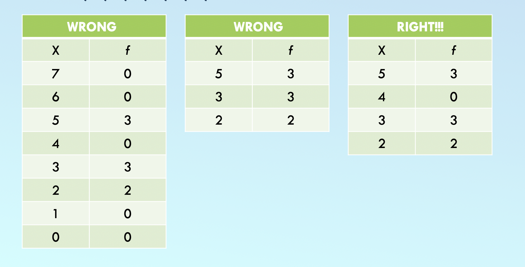
The tables consist of at least 2 columns:

• X column = X values from high to low. These only include values within the range of your scores.
• ƒ (frequency) column - tallies (or frequencies) are determined for each value. Tells how much each X occurs in the data set

ƒ says “how many people in our dataset have this value

The sum of frequencies = N or n

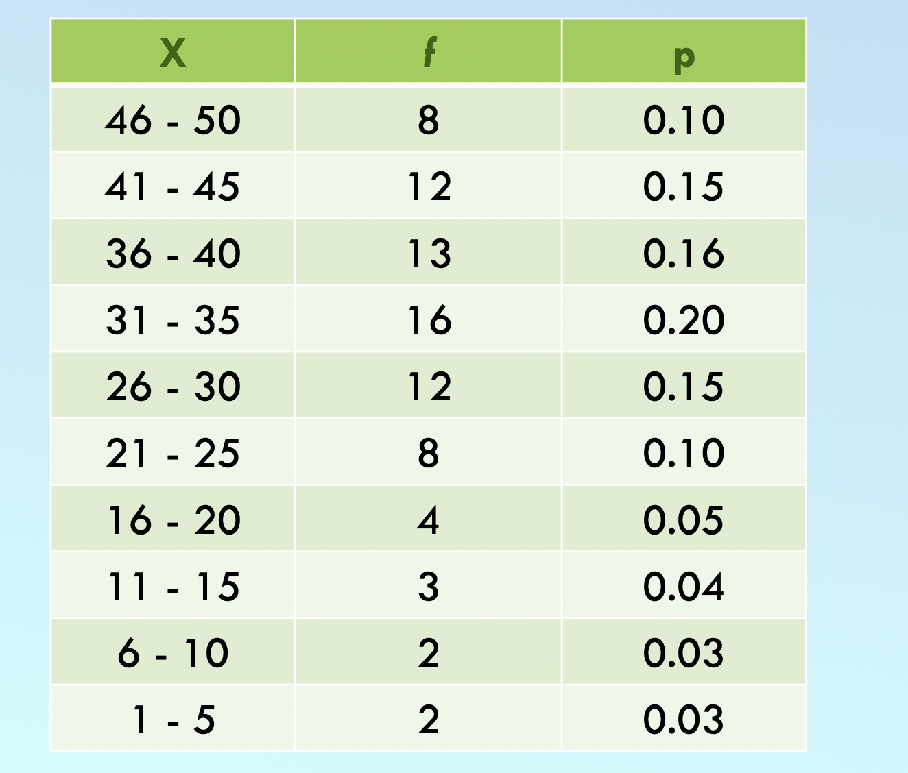
Group frequency distribution: Used when listing all X values would be too long

• Lists groups of scores rather than individual scores
• Groups of scores are called Class intervals. These intervals have the same “width” (usually a simple number ; 2,5,10 points etc)
• Interval width is selected so that the table will have 10 intervals usually
• p= proportion for each category

Caluclated by p= ƒ/N

Example:

Frequency distribution Graphs:

• X values are on x-axis
• Frequencies are on y-axis
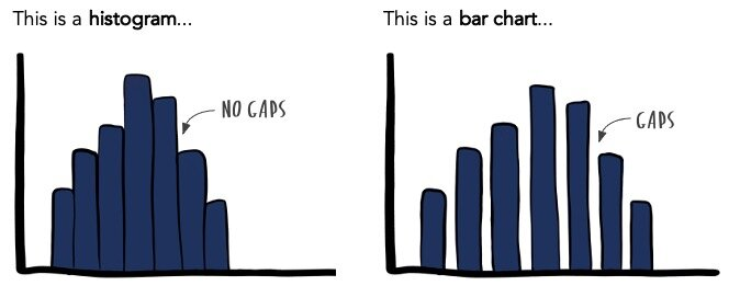
• When score of categories are on an interval or ratio scale, graph should be either a histogram or a polygon (Not a bar graph). Be able to read these ! Used for interval or ratio scales

Example:

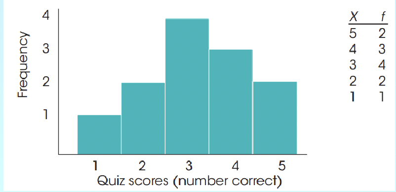
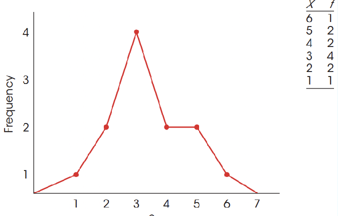
(Histogram) (Polygon)

Bar graphs:

• Must be used if you have nominal data
• When X values are on a nominal or ordinal scale
• Just like a histogram but the gaps are left between adjacent bars
• Nominal scales: space between the bars are used to say that categories are separate; distinct
• Ordinal scales: uses separate bars because you cannot assume all the categories are all the same size

Smooth curves:

• Used for when a population consists with scores from an interval or ratio scale
• Indicates the relative changes that occur from one score to the next. You are not connecting a series of dots (real frequencies)
• Representing data in the population
• Histogram/polygon is used in samples (when interval or ratio)

Normal curve:

• Contains a symmetrical curve with highest frequency in the middle and relative frequencies decreasing as you approach either extreme

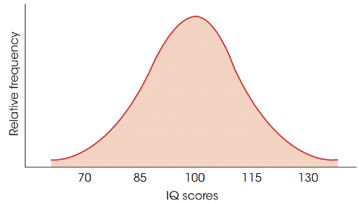
Displays a lot of IQ scores in the middle

Types of distributions:

Normal distribution: a symmetrical distribution with greatest frequency in the middle and middle frequencies decreasing as you move away from the middle in either direction. Occurs a lot in data because there are multiple determinants ; generally things tend toward the middle and fewer observations of extremes

Shapes of distributions:

Symmetrical distribution: possible to draw a vertical line through it so that one side of the distribution is the mirror image of the other.

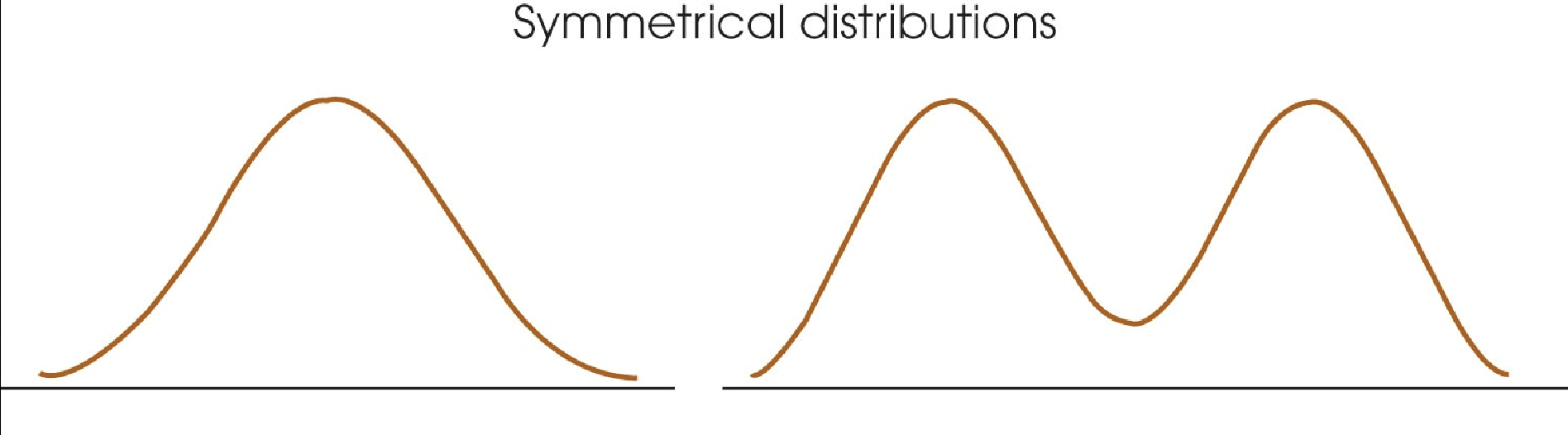
Hill shape or 2 hill shape (both symmetrical)

Skewed distribution: Scores pile up on one side of the distribution leaving a tail of a few extreme values on either side.

• The section where scores taper toward one end of the distribution is called the tail of the distribution

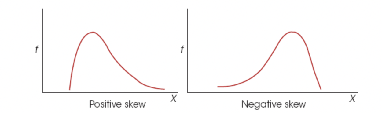
(tail points on positive end) (tail points on negative end)

Stem and Leaf displays: efficient method for displaying a frequency distribution

• Requires each score be separated into 2 parts
• First digit is called the stem and the last digit is called the leaf

Example: 67 stem is 6 leaf is 7

• All stems all go in one column and leafs in another
• This allows you to view every individual score in the data
• # of leafs beside eacg stem represents the frequency for that interval
• Individual leafs identify individual scores
• Only useful for small samples/populations because each score is listed***

Percentiles & Percentile ranks: Where you stack up in the distribution

• Relative location of individual scores in a distribution (used a lot in hypothesis testing)

Percentile rank: The percentage (%) of individuals with scores equal or less than a given X value. (Ex: if you earn the 2nd highest SAT score in a class of 100 your percentile rank = 99%

Percentile: When an X value is described by its rank

CHAPTER 3:

Central Tendency: The concept of an average or representative score that most represents the entire group. A statistical measure that uses a single value to describe the center of the distribution

• Attempts to identify the single value that best represents the entire dataset; can be used to describe an entire sample or population
• Useful for making comparisons between individuals or sets of data by comparing the average score
• Makes large amounts of data more digestible; condensing it into a single value
• A descriptive stat (describing data in a simple concise form
• There are many ways to determine this value but no single procedure produces a good representative value: Mean, Median, Mode.

The Mode: The most frequently occurring score or class interval in the distribution

• In a graph, the mode corresponds to the highest point in the distribution
• Works with nominal, ordinal, interval, or ratio data (alll scales of measurement; mostly for nominal)
• The only measure of central tendency that can be used for data measured on a nominal scale
• Often also used as a supplemental measure of central tendency for ordinal, interval or ratio data–reported along w/ median or the mean

Bimodal Distributions: possible to have more than one mode **systematic decrease and ascend**

• 2 modes = bimodal
• 3 or more modes = multimodal
• Different from central tendency bc the distribution can have only one mean and only 1 median
• The general term ‘mode’ is also used to describe a peak in a distribution that is not necessarily the highest point

Major Mode- Highest peak

Minor Mode- secondary peak ; Used when distribution is clearly humped.

Normal Bimodal

The Median: Divides the score so that 50% have values equal to or less than the median

• If scores are listed smallest to largest, the median is the midpoint of the list
• Requires scores to be placed in rank order. CANNOT be done with nominal data. ONLY works with ordinal, interval or ratio scales
• If there’s an odd number of scores, median = middle
• If even, add middle scores and divide by 2
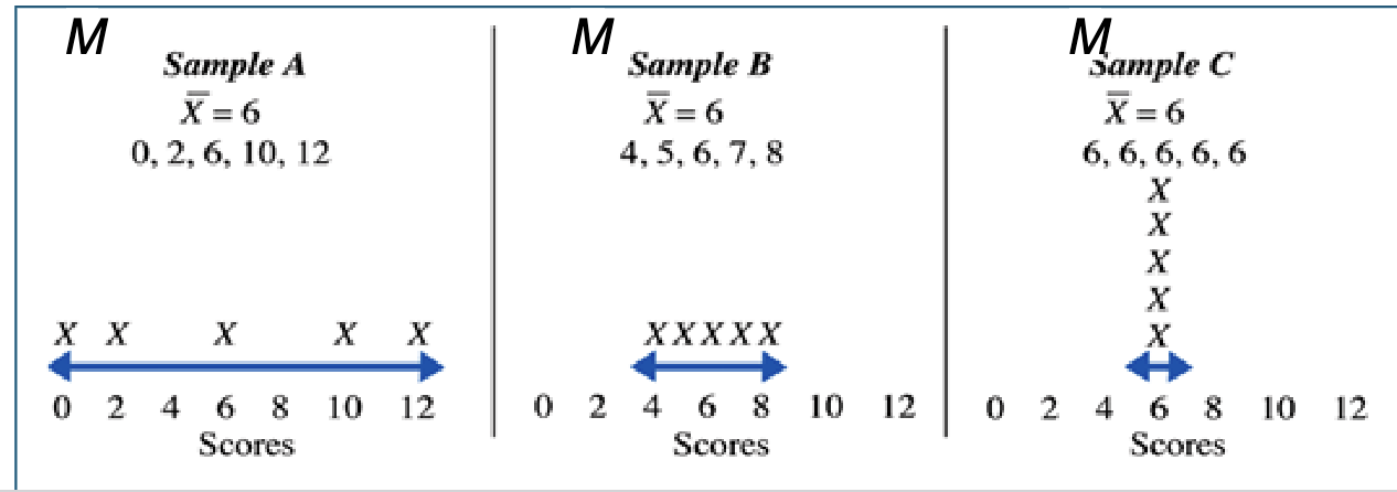
• Relatively unaffected by extreme scores
• Tends to stay in the center even when there are extreme score or the distribution is very skewed; in this situation, median is a good alternative to the mean

The Mean: the arithmetic average

• Computed by adding all the scores in the distribution and then dividing by the number of scores
• For a population, mean = μ uses greek letters
• For a sample, mean = M or x̄ (X-bar) uses regular letters
• Most commonly used for ordinal, interval or ratio (best for interval or ratio because same increments)
• Sum of the distances below the mean is exactly equal to the sum of the distances above the mean
• Accounts for magnitude of difference (preserves that about the scores unlike the median)

Population mean: 𝞢X/N

Sample mean: 𝝨X/n

Alternate definitions for Mean:

Dividing the total equally

• The amount each individual receives when the total is divided equally among all the individuals (N) in the distribution

The Mean as a balancing point

Mean Characteristics

• Changing the mean: bc calculation involves every score, changing the value of any score will always change the mean
• Discarding or adding new scores: will almost always change the mean EXCEPT for when you add or discard a score that is equal to the mean
• If a constant value is added or subtracted from that score → the mean is increased or reduced by that same constant value
• If every score is multiplied or divided by a constant value → the new mean = old mean multiplied or divided by that same constant value

Situations when the mean doesn't work:

• When distribution contains a few extreme scores (Like US income); the data skewed
• Very skewed (also like US income)
• This causes mean to be pulled toward tail or toward extreme scores; this means mean will not provide central score
• When distribution is “humped”
• When data is nominal scale, it’s impossible to compute a mean for that data

Central Tendency and the shape of the distribution

• In a symmetrical distribution, the mean and median will always be equal
• If the distribution has 1) 1 mode AND 2) it is symmetrical, the mode will also be equal to the mean and median; if data has one mode but not symmetrical, it will not be equal to the mean and median

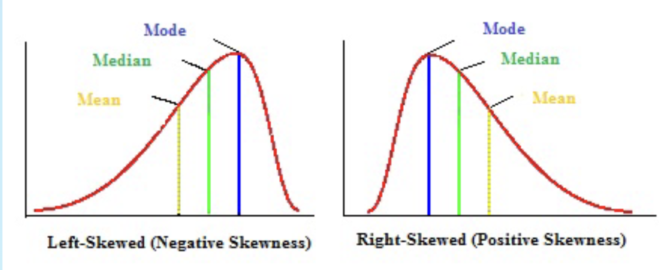
In a skewed distribution:

• The mode will be located at the peak on one side
• The Mean usually will be displaced towards the tail on the other side
• The median is usually located between the mean and the mode

CHAPTER 4

Variability: helps you figure out what’s going to happen

• Refers to how much scores in a dataset differ from each other

Why measure it:

• Describes the data set’s distribution (clustered vs. spread out)
• Also tells us how well an individual score represents the data set

High variability low variability no variability

Variability: How scores are scattered around the central point

Measuring Variability:

Can be measured with…

• The range
• The variance/standard deviation
• In both cases of range and standard deviation, variability measures the distance

The range: Indicates the distance between the most extreme scores in a data set

• Range (v1)= Highest score - lowest score
• Range (v2)= lowest score and highest score (ex; range: 3-9 ; 3 to 9)

Range limitations:

• It’s useful as a very rough approximation of variability
• However, it is an imprecise and unreliable measure because it is based on 2 scores; not all scores are represented

Central tendency should be to compare each score to the Mean; considering all scores

Differences from the mean should be squared so that the different scores are always positive

Variance and standard deviation:

When using mean: Use variance and standard deviation to describe variability in the data

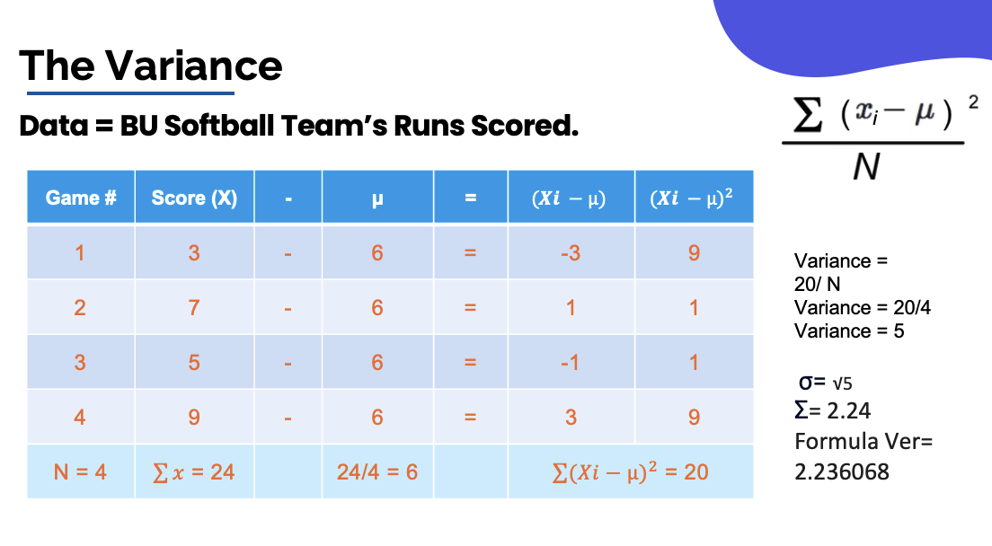
Variance= the average squared deviation from the mean

Standard deviation: the most common measure of variability

• Measures the average distance from the mean for scores in the dataset
• Variance determines the standard deviation

4 steps for calculating standard deviation:

Step 1: determine each scores deviation (AKA distance from mean)

• Deviation score = X_i - μ

Step 2: Square the deviations (so it is not zero)

Step 3: Find the average of the squared deviations

• Do this by the sum of the squared deviations (This is called the Sum of Squares)
• Average the squared deviations (giving you the variance)

Step 4: Take the square root of the variance

• The standard deviation is just the square root of the variance
• Standard deviation (σ = √variance)

Common Mistakes:

Mistake #1: squaring raw scores

Correct: square the difference scores

Mistake #2: summing different scores then squaring them

Correct: square each different score, THEN sum.

Standard deviation self-check:

• The standard deviation can never be less than the distance between the mean and least deviant score
• It can’t be negative
• It can never be greater than the distance between the mean and the most deviant score

The standard deviation formula for samples is slightly different than its formula for populations (and notation)

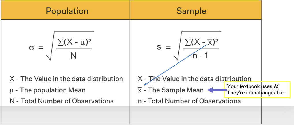
Dividing by N-1 is the only difference!

Notes about n-1:

• For samples, we divide n-1to inflate estimate of variance (bringing it back in line with what happens in the real world population)
• N-1 is the degrees of freedom (dƒ) for S
• Accounts for the fact that sample variance will typically underestimate population variance
• This effect is stronger with smaller samples and the effect of dƒ help account for that too

Properties for standard deviation:

• If a constant is added or subtracted to every score, the standard deviation will not be changed

(Shape does not change, just mean)

• The spread (or variability) doesn’t change
• If each score is multiplied or divided by a constant the standard deviation will be multiplied or divided by that same constant
• It will multiply the distance between the scores and the standard deviation measures this distance

What standard deviation can tell you:

• Mean & standard deviation do a good job of describing most distributions; particularly if there isn’t much skew
• If you are given mean and standard deviation….you can construct a rough sketch of the distribution
• Application problem:
• You add two random observations. If the total is 120 or greater you get 1k
• Sample1:M=25 S=10
• Pick this: Sample 2: M =40, S =45 (Variability is higher so there is more of a chance to get scores above 60

CHAPTER 5

Z scores = SD scores

• Z scores are just a way to express data in terms of the mean and standard deviation
• A Z-score tells us how far away the point is from the mean as a proportion of the standard deviation

+1.00= 1 SD above the mean

• By itself, a raw X value provides little information.

For example, X=106 may be low, average, or very high depending on the mean and standard deviation

• If the raw score is transformed into a z-score, the value tells exactly where the score is located relative to all other scores

Z-Scores and location

A Z-score is a X-score that has been transformed such that:

• Sign (+ or - ) identifies whether the X score is located above or below the mean (which side)
• It’s a numerical value- the number of standard deviation units between the X and the M (magnitude) (Ex a z-score = -1.00 tells ys the score is 1 s (standard deviation) below the mean

Transforming From X to Z

z = X - μ / σ

z= X- M / s

Remember ***

• Z-scores always consist of two parts (1. A sign (+ or -) 2. A magnitude
• All z scores above the mean are positive
• All z scores below the mean are negative
• The numerical value of the z-score tells you the number of standard deviations from the mean
• A z-score of 0 is equivalent to the mean
• Z = 0 = μ or M
• Because it’s telling us that the score is 0 standard deviations from the mean
• Although more extreme z-scores do occur, the majority of the distribution (958%) exists between z = -2.00 and z= +2.00

Transforming from Z to X

Find the center point based on the mean, then multiply the magnitude to get back to the X value

Population : X = μ + zσ sample : X = M + zS

Example:

z = +2.50, < = 15, s = 10

zs = 2.5 *10 = 25

X = M +zs = 15+25=40

= -0.50

Z scores are descriptive and inferential statistics….

Descriptive: They describe exactly where each individual score is located

Inferential: they can determine whether a specific sample is representative of a population

• Can also tell you if a specific score is representative of a sample

Z-scores above or below 2 are typically considered extreme/unrepresentative (the top and bottom 2%)

Z-scores as a standardized distribution

• To create a standardized distribution transform each x-score into a z-score
  • Use the same formula discussed earlier
• Distribution will always have M = 0 and S = 1 (once each x-score is converted into a z-score)
• This does NOT change the shape of the raw distribution; just makes more meaning of the numbers easier to read
• Does NOT change the location of any individual score relative to others
• All that changes is the scale.

Advantages of standardizing

• You can compare distributions with different scales
  • Example: Pop A = μ = 100 and s = 10
  • Pop B : μ 40 and std =
• When transformed into z scores
• Pop A and B will both have mean of 0 and std of 1
• Now compare relative distance from mean

Using Z-Scores to transform distributions